10 Interpreting Model Coefficients

Last chapter we began building and automatically fitting statistical models of a data generation process. When we did so, by specifying our assumptions for the prediction equation and observation model, we got back coefficient numbers which maximize the likelihood of the data given our model form. After verifying that this form of the model fit the data reasonably well, we can look at these coefficient values and interpret them.

We want to interpret them because these aren’t just superfluous calibration numbers - they mean something about the data generation process we are studying, and understanding them helps us understand the role of the explanatory variable(s) in our model. In this chapter, we will explore in more detail how to interpret these values in the prediction equation. In Chapter 11, we will cover interpretation of the values in the observation model.

10.1 Line of best fit

Let’s go back to our research question from last chapter: the relationship between number of siblings and education attainment. Our research hypothesis was that more siblings would be associated with less education, and we first made a scatter plot to visually look at this association:

We thought we saw a negative association, because it looks like the conditional probability distribution of education attainment is shifting downward as number of siblings increases. We can highlight this more clearly in our scatter plot by adding a layer of red dots that represent the average education attainment for each number of siblings:

The stat_summary() function we used is a ggplot() option for summarizing something about the data in the plot, and adding that summary as a layer to the image. In this case, we specified the summary to be the mean (fun=mean argument), and the summary is plotted as a large red point (geom="point", color="red", size=4 arguments). We chose to visualize the mean because that is the parameter of the target variable that we think the explanatory variable will influence.

Now, it is clearer that the average education attainment is decreasing as number of siblings increases. This is consistent with our verbal proposal about the data generation process of education attainment. But as we discussed at the end of last chapter, we should specify a formal model of this system to make the idea quantifiable and testable. So how do we go about turning what we see into numbers?

We could start by writing out what we would predict about the mean of education attainment for one specific value on the explanatory variable, number_of_brothers_and_sisters = 0. On the graph, it looks like that is a little bit under 15 years of education, so we could write that as something like $\mu_{P(Y|X=0)} = 14.7$. Now looking at another value, e.g. number_of_brothers_and_sisters = 5, our prediction is different - something like $\mu_{P(Y|X=5)} = 13.3$.

We could keep going like this, essentially writing out the prediction equation as a verbose list of predictions: $\mu = \{14.72, 14.45, 14.18, ..., 12.02\}$ for $X = \{0,1,2,..., 10\}$. But that is not a very efficient way to describe the data generation process - it’s not parsimonious. It might not even be possible to do, if our explanatory variable was something continuous with infinite decimal value possibilities rather than discrete integers.

Let’s try a slightly different strategy instead. Looking again at where the red dots are - it kind of looks like they’re forming a line, doesn’t it? Remember from geometry class that there is a simple equation that describes how to draw a line on a plot:

\[y = mx + b \tag{10.1}\]

If we plot a line like this on our scatter plot:

The line doesn’t perfectly overlap with all the mean points, but it’s a pretty good approximation for a lot of them. This is known as the line of best fit through the data. So, if we want a simple equation we could use to predict outcome data based on explanatory values, the equation for the line of best fit is a good candidate.

Using the equation for line of best fit has a couple of benefits. First, rather than writing a bunch of individual values for each unique value of $X$, there are just two important pieces to this equation: $b$, where the line crosses the y-axis (value of $y$ when $x=0$), and $m$, the slope of the line (rate of rise over run). This is much simpler to write! If we use this equation form for the prediction equation, we do a pretty good job of predicting the means of the conditional probability distributions while keeping the model parsimonious and easier to work with.

Just a few unknown coefficients also makes it easier for the computer to find the optimal values during fitting. Sometimes, if there are a lot of coefficients to search for, there might not be enough data available to fit the model well. The model fitting procedure will select values that work for these specific points, but wouldn’t work for other points if we collected more data. This situation is called overfitting. If there are more coefficients than there are data points, the model fitting procedure can’t even find values to use because there are too many unknowns relative to known information.

overfitting = when a model fits the training data too closely and fails to generalize to new data

Figure 10.1: Two examples of fitting a statistical model to a sample of data with a linear prediction equation vs. something more complicated. Black dots are the sample of data, while red dots are the target means at each level of X in this sample. The model on the right fits this particular sample of data really well, but doesn’t generalize to the wider population of data (gray dots) as well as the simpler line.

Lastly, the equation for a line is useful for predicting new data. If we used our long list of target means to make predictions about education attainment for someone new who had 0 siblings, we could use the mean of everyone else we recorded with 0 siblings (14.72 years of education) as our prediction of the most likely value. But if someone comes along with a number of siblings that no one else in our dataset has, what would we guess? When using the line of best fit, we could still predict a value for this person by simply plugging in the new sibling number for $X$ in the equation. Being able to make predictions about data that we haven’t actually observed yet makes this approach useful for prediction research goals.

10.2 The General Linear Model

Because of the advantages discussed above, using the equation for a line of best fit as the form of the prediction equation in a statistical model is really common. In fact, it has a special name: the General Linear Model (GLM). ¹.

General Linear Model = a statistical model where the prediction equation takes the form of a linear equation.

The “linear” part of the name comes from the fact that we are using the equation of a line through our data². In other words, we are assuming a linear and monotonic relationship between the explanatory variable and the parameter of the target variable distribution.

The “general” part of the name comes from the fact that the general equation form applies to lots of different model ideas: multiplying the variables by different coefficients, adding more variables into the mix, or predicting different parameters of a target distribution. All of those adjustments are still writable in the same general equation form.

Before we know the exact values of the coefficients, we can refer to this equation form by writing:

\[ \mu = \beta_0 + \beta_1X \tag{10.2}\]

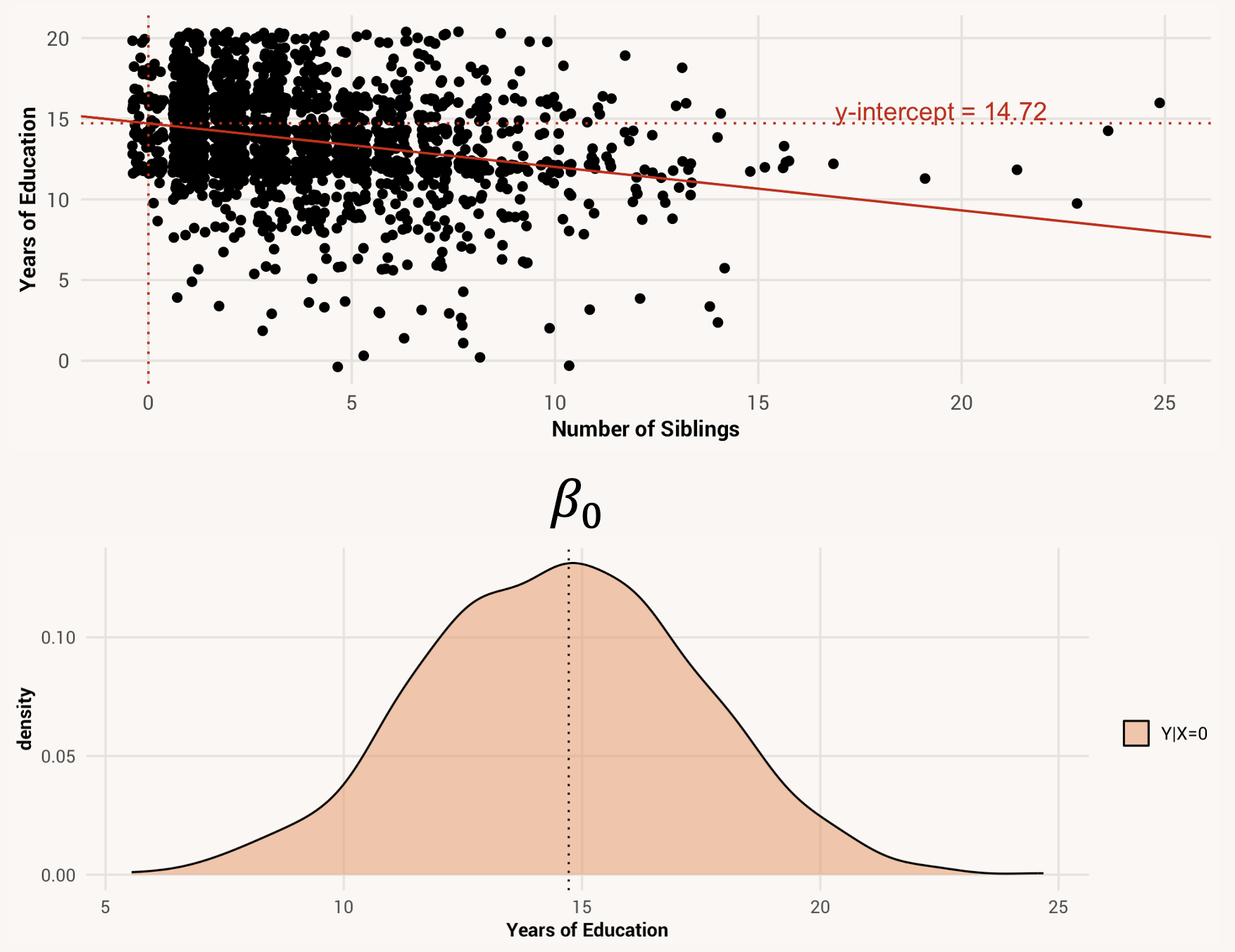
This is the canonical notation for the GLM equation. It’s just a rearrangement and relabeling of the line equation pieces. $\beta_0$ stands for the y-intercept. More concretely, it is what we would predict for the $\mu$ of the target variable when the explanatory variable is 0. This is because $\mu = \beta_0 + \beta_1*0 = \beta_0$, with the second piece dropping out of the equation when multiplied by 0.

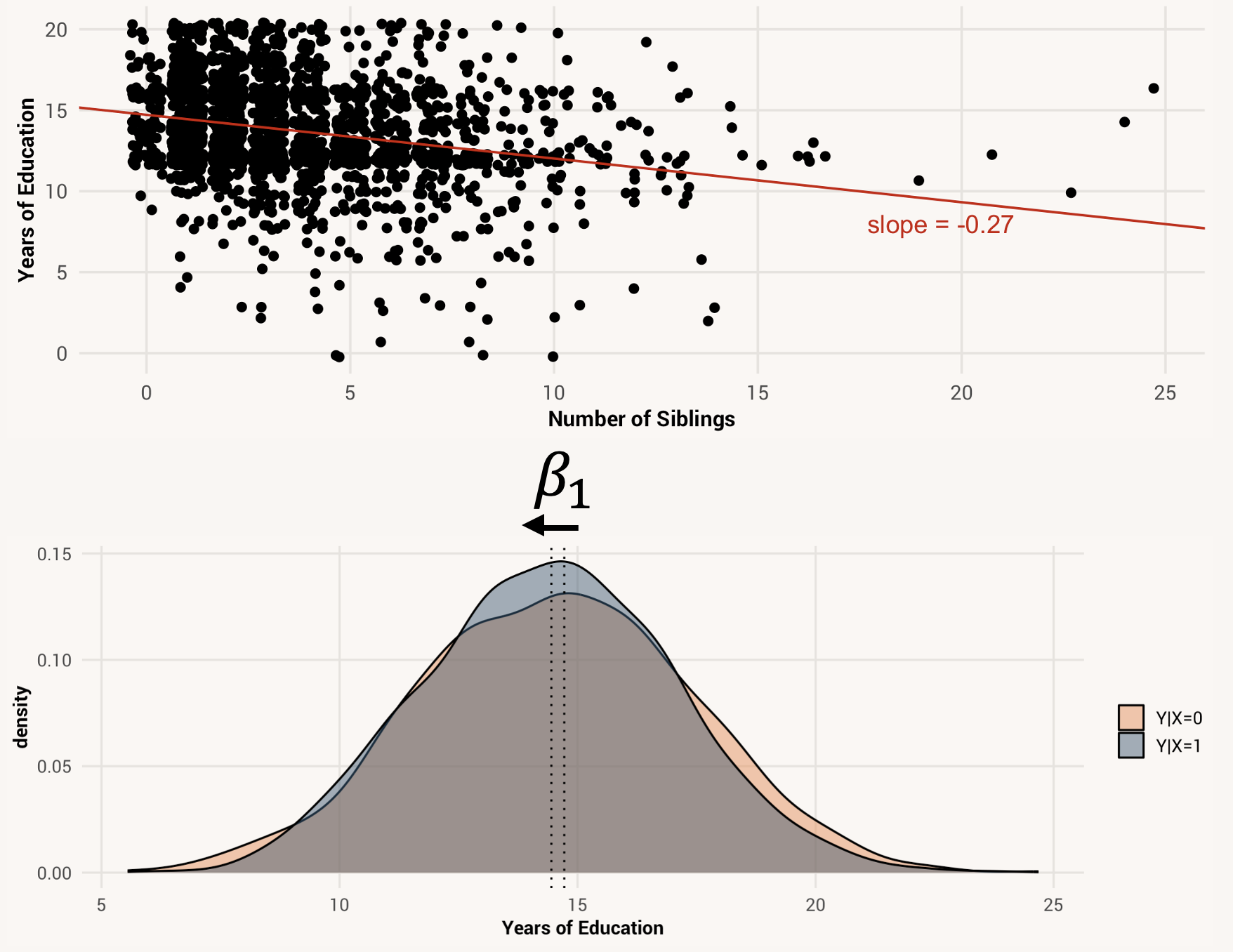
$\beta_1$ is the slope of the best fitting line through the data. This is the change in the target mean for every 1-unit increase in $X$. Another name for this number is the effect of $X$ on $Y$³. We would say $X$ has a large effect on $Y$ if $\beta_1$ is a big number - a 1-unit change in $X$ results in a large change in the parameter of $Y|X$. If $\beta_1$ is small, however, there is only a small effect of $X$ on $Y$ because the parameter of $Y|X$ doesn’t change very much when $X$ does.

effect = the magnitude of change in the target variable parameter associated with a one-unit change in the explanatory variable

10.3 Interpreting model coefficients

Let’s practice finding and interpreting these values in a fitted statistical model.

Exercise

In the code cell below, fit a general linear model where the target variable is highest_year_of_school_completed and the explanatory variable is number_of_brothers_and_sisters in the gss_clean dataset.

We see the table of coefficients in this output (alternatively we could have looked at these numbers by typing model$coefficients). Which number is $\beta_0$ and which is $\beta_1$?

Now that we know that $\beta_0$ represents the y-intercept of a line of best fit, it makes sense why one number is labeled (Intercept). This number is the best $\beta_0$ value for our data. We interpret it as telling us that our prediction equation expects there to be an average education level of 14.72 years for people with 0 siblings.

Figure 10.2: Mean of P(Y|X) when X=0, i.e. the y-intercept.

The next number, labeled with the name of the explanatory variable, is $\beta_1$. We interpret this number as the effect of that explanatory variable on the conditional probability of the target. It is the steepness of the slope of the best fitting line.

Another way to think about the effect of the explanatory variable is as a comparison - how much different is the expected outcome for people with 0 siblings vs. people with 1 sibling? For every 1-unit increase in number of siblings, we expect the mean education level of people in the dataset to decrease by -0.27 years. This is because $14.72 + (-0.27)*1 = 14.45$, which is 0.27 less than the mean education for 0 siblings.

Some things to keep in mind about the coefficient interpretations we’re making right now. First, we can think of these values as estimates of estimands we may be interested in. If we had been interested in the relationship between education and number of siblings, the model gives us a specific answer: -0.27 years per sibling, assuming a linear association with no other explanatory variables. Or maybe we had a prediction goal and wanted to know what level of education to expect about someone with no siblings. In this case our estimand is the expected education level when $X=0$, which is $\beta_0$ in the model. 14.72 years on average is the estimate of this estimand. Our estimand can also be about something that’s not one of the coefficients, but the coefficients can help us get there: e.g., if I have 4 children, what is my expectation for how much education my children will get? The fitted model equation tells us how we can calculate an estimate of this estimand: 14.72 + (-0.27)*3 = 13.91 years of education for my children on average⁴.

Also, our interpretations are what these numbers mean for the target parameter we are modeling, and are thus specific to that parameter. In this data generation process, we hypothesized that the mean of education would change as a function of number of siblings, so we fit a prediction equation $\mu = \beta_0 + \beta_1X$ to encode our ideas of the data generation process and generate an estimate for that quantity. But if we had hypothesized that something else about the target variable was affected by the explanatory variable, e.g. $\sigma = \beta_0 + \beta_1X$, then the model fitting procedure would optimize for what $\sigma$ values of $Y|X$ make the data most likely and would find different coefficient values. The ones we found in this example, then, are specific to how the target mean changes as a function of $X$. If we wanted to examine the hypothesis about $\sigma$ instead, we’d need to fit a different model, get different coefficients, and interpret those relative to changes in $\sigma$ specifically. In this way, a coefficient does not have meaning in isolation - its interpretation depends on the larger context of whole model of the data generation process.

Third, notice that we are interpreting these numbers in terms of the units of the variables. $\beta_0$ is in units of years of education. That’s the units of the target variable, and we use the same units to talk about the target’s mean. $\beta_1$ is in units of years of education per sibling. This is because when $X$ changes by 1 in the equation (increase in 1 sibling), $\mu$ changes by $\beta_1$. The effect of $X$ on a parameter of $Y|X$ is expressed in terms of how many units the parameter of $Y|X$ changes by per unit of $X$.

Lastly, the coefficient values make the data we currently have most likely to occur under the proposed statistical model, and thus reflect how the parameter of the conditional probability distribution changes for these data. But that doesn’t mean they would be the best coefficient values in a different dataset! Remember all the way back in Chapter 1 when we discussed that part of asking a good statistical question is knowing which population you are asking about. The population we are modeling right now is the population these data were collected from - adults in the US. The data generation process of education attainment could be different in different countries - a different mean level of education for people with no siblings for instance, or a weaker/stronger effect of sibling number. We don’t have access to data from other populations to know that, however. So we have to restrict our interpretations of the data generation process to what they mean for this population we do have data from. This is why, for researchers interested in the fundamental processes of human cognition, it is really important to sample from all humans.

10.4 Modeling with a categorical explanatory variable

So far we have defined, fitted, and interpreted one particular statistical model of a data generation process: the influence of number of siblings on someone’s education level. These were our variables of interest and the size of the influence was our core estimand for a broader research goal of explaining what influences education outcomes. We defined our statistical question this way, and the modeling procedures followed.

Imagine we now have a different estimand we care about: how years of education depend on respondent sex. Let’s go through the steps of the modeling workflow we’ve learned so far to see how we would model this data generation process in order to find an estimate for our estimand.

First, we need to make guesses for each component of the data generation process. Component 1, what comes out, is going to be the same target variable we were working with before: highest_year_of_school_completed. Thus the nature of this variable (interval scale) will be the same. Also, this is probably still a probabilistic data generation process, so the output of the model is a probability distribution of this data rather than exact values.

Next, component 2 is the explanatory variable(s). Our hypothesis is now that respondent sex, male or female, will influence education attainment. This means the respondents_sex variable in gss will be our explanatory variable.

Thirdly, what is it about education that we think sex will influence? Since we said this is a probabilistic data generation process, sex should influence some parameter of education’s conditional probability distribution. Let’s say our hypothesis is that males will tend to have higher education than females on average, which means the parameter we think is influenced by the explanatory variable is again the mean of highest_year_of_school_completed, $\mu$.

Finally, we need to specify the form of the prediction equation. We can still use the GLM form here.

Altogether, the equations of our model are:

\[Y \sim \mathcal{N}(\mu, \sigma)\]

\[\mu = \beta_0 + \beta_1X\]

Next, we automatically fit this model to achieve coefficient values. Our chosen observation model tells us which fitting function to use and our chosen prediction equation tells us how to write the formula argument.

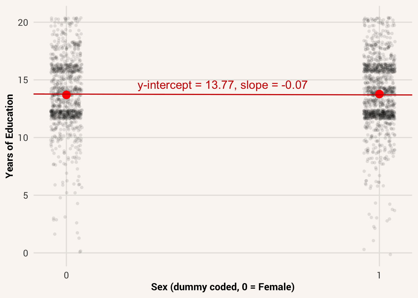
Looking at the coefficient values, we see that $\beta_0$ is 13.77 and $\beta_1$ is -0.07. This indicates that the mean education value for someone with respondents_sex = 0 is 13.77 years, and the effect of sex on education is -0.07 years per unit increase in respondents_sex.

But wait - before we read into the answers too much, we should check how well a data generation process of this form would create data like those we observed. If there isn’t a good fit, we should reevaluate our idea about the prediction equation form or observation model family. We simulate data using the coefficient values, and inspect the simulated distribution compared to the observed target distribution.

Hang on, this is the same simulation we did in Chapter 9 - why is there now an error?

The text of the error gives us an important clue: Error: non-numeric argument to binary operator. This is telling us that R can’t evaluate this code as math, because gss_clean$respondents_sex[i] is not numeric. Indeed,

It is a character data type.

In order to use this variable in math, we need to turn it into a dummy variable. We first learned about this idea is Chapter 5. To review, a dummy variable quantifies a binary categorical variable by assigning one category label as “0” and the other as “1”. Here is the same simulation code, but with respondents_sex converted to a dummy variable:

Now we have a working simulation, and indeed it looks like there’s decent agreement between the central tendency and spread of the simulated data compared to that of the real dataset⁵.

Why didn’t we need to do this dummy operation when first fitting the model? In fact, we did, but R’s lm() function is smart and automatically did it for us under the hood. R also gives us a simulation function, predict(), that can do this for us as well so we don’t have to handle the dummy coding ourselves. predict() takes two arguments, the fitted model object to refer to (object= argument) and a vector or data frame of data to predict for (newdata= argument). The explanatory variable(s) in the new data must exist in this data frame with the same variable names as those in the data used for model fitting. The output of this function is whatever the prediction equation in our model would calculate.

Here is an updated version of our simulation code, using predict() on line 6 instead:

Now that we feel satisfied with how well the model form fits the data, we can return to interpreting the model coefficients. However, since we interpret the coefficients in terms of the variable units and we know that the explanatory variable is now a dummy variable under the hood, we should adjust our interpretations a bit. $\beta_0$ is still the mean of the target variable when the explanatory variable is 0 and $\beta_1$ is still the change in this mean for a 1-unit increase in the explanatory variable. But what does it mean for this specific explanatory variable to be 0, or to change by 1 unit?

Since respondents_sex was dummy coded, a value of 0 corresponds to people who are in the category assigned the “0” label. When doing dummy coding ourselves, we chose that assignment in the way we wrote the arguments of recode_values(): by writing from = c("Female", "Male") and to = c(0,1), we assigned the first category (“Female”) to be the first numeric value (0) and so forth. When we let lm() do the dummy coding, it automatically picks whatever category comes first in the alphabet to be 0. In this case that also makes “Female” be 0. Altogether, this means that we should interpret $\beta_0$ as the mean of highest_year_of_school_completed for people with $X=0$, i.e. female respondents. The group that is assigned to a label of “0”, and thus has $\beta_0$ as its mean, is known as the reference group in the model.

reference group = the category of a categorical explanatory variable that is assigned a value of 0 when dummy coding, and to which other groups are compared

A 1-unit change in X is the process of switching groups - going from 0 to 1. The meaning of $\beta_1$ is then the change in the mean of highest_year_of_school_completed when going from the reference group to the comparison group (female to male respondents). Female respondents on average have 13.77 years of education ($13.77 + -0.07*0 = 13.77$), while male respondents on average have 13.70 years of education ($13.77 + -0.07*1 = 13.70$). $\beta_1$ is the difference between the mean education levels of the two groups, with male respondent education being slightly lower than that for female respondents. Looks like our hypothesis (that male respondents on average have higher education than female respondents) wasn’t supported by these data.

Note how we didn’t have to change the prediction equation to accommodate a categorical explanatory variable. The equation form $\mu = \beta_0 + \beta_1X$ still works for categorical variables as long as we can dummy code them. This flexibility illustrates the “general” part of the General Linear Model, and why it is so commonly used. The general meaning of the coefficients also stayed the same - $\beta_0$ is still the y-intercept and $\beta_1$ is still the slope of the best fitting line. We just had to interpret what these quantities mean in the context of the specific variables we chose.

Figure 10.3: Line of best fit through the means of each category of Sex (Female = 0, Male = 1).

10.5 Standardized coefficients

When we interpret coefficients in terms of the variable units, that is helpful for us to understand how big of a consequence the explanatory variable has on the target variable. In our example using number of siblings as the explanatory variable, an effect of -0.27 years of education per sibling means that having 4 siblings vs. 0 could determine whether someone stops going to college one year earlier ($14.72$ vs. $14.72 - 0.27*4 = 13.64$). If we’re using this model for prediction or explanation goals, that effect size can inform us about what education levels to expect in a society with certain family planning trends, or how much public policy investment we need if we hope to increase education attainment by a certain amount.

However, this decision-making about the meaning of the coefficients is only possible if we understand what the units of the variables mean. Years of education and number of siblings are variables and units we encounter in our everyday lives, and we have existing instincts about what big and small values are on those variables. But what if we were studying something more abstract like brain activation? If we said the effect of stimuli orientation on brain activity was -0.27 amplitude per radian of rotation, is that a big or small effect in the context of those variables? Have you even heard of those words before?

Or, what if we were studying the effect of number of siblings on education but we had measured education in terms of months instead of years? The same effect of -0.27 years per sibling would be -3.24 months per sibling, which is a bigger number even though the effect itself is the same. If we were trying to compare the size of the effect we found in the US vs. Germany, but one study had measured education in terms of years and the other in terms of months, it would be hard to understand if the effects were the same. The conversion is more obvious in this example, but you can probably think of others where the measured variables are more abstract, like different survey instruments targeting social anxiety. It’s not clear how to translate between these different scales when they don’t have interval measurement.

Because of these realities, sometimes it is not the most helpful to interpret model coefficients in terms of the variable’s original units. Sometimes it is instead better to look at standardized coefficients.

standardized coefficient = a statistical model coefficient that has been transformed to be in terms of standard deviations of the variables rather than their original units

10.5.1 Standardized model coefficients with an interval explanatory variable

We used z-scores in Chapter 5 and correlation in Chapter 6 to understand the magnitude of distributions and associations generally, separate from the specific units of the variables. To do this we divided statistics by the variation in the variables used to compute them. This essentially brings all variables into the same, unitless scale.

We can do the same with our statistical model coefficients to standardize them. We simply model how the z-scored values of the explanatory variable influence the mean of the z-scored target variable distribution.

Exercise

Fit a general linear model with the standardized forms of the variables highest_year_of_school_completed and number_of_brothers_and_sisters.

Now we have very different coefficient values. Let’s walk through what they mean relative to the new standardized units of the variables.

The intercept, $\beta_0$, is a really tiny number. This is essentially 0. Remember that $\beta_0$ is the mean target value when the explanatory variable is 0. Since we z-scored number_of_brothers_and_sisters, a z=0 value on this new variable corresponds to the mean of number_of_brothers_and_sisters. Because the y-intercept value is 0, we predict the most likely education value will be the marginal mean $Y$ when at the mean of $X$. Someone average on one variable is expected to be average on the other.

Figure 10.4: Mean of P(Y|X) when X=0 and variables are z-scored.

The $\beta_1$ value, -0.26, tells us how to adjust our predictions from there. A 1-unit increase in a z-scored variable is an increase of 1 standard deviation in the original variable. We should interpret a standardized $\beta_1$ value as the change in $Y|X$’s mean per unit of $X$, so here we say that a 1SD increase in $X$ is associated with a -0.26SD decrease in the mean of $Y|X$.

There are actually multiple ways we could get to this standardization. Z-scoring the variables first before fitting a model is one way, but we could also fit a model with the original variables and then convert the raw $\beta_1$ value. Since $\beta_1$ is the change in $Y|X$’s mean per 1-unit increase of $X$, and 1 standardized unit of $X$ is $s_X$, the expected change in $Y|X$ per 1 standardized unit of $X$ is $\beta_1 * s_X$. To express that in terms of standardized units of $Y$, we divide by $s_Y$. This gives us a formula for converting an unstandardized coefficient to a standardized one:

\[\beta_1^{std} = \frac{\beta_1 * s_X}{s_Y}\]

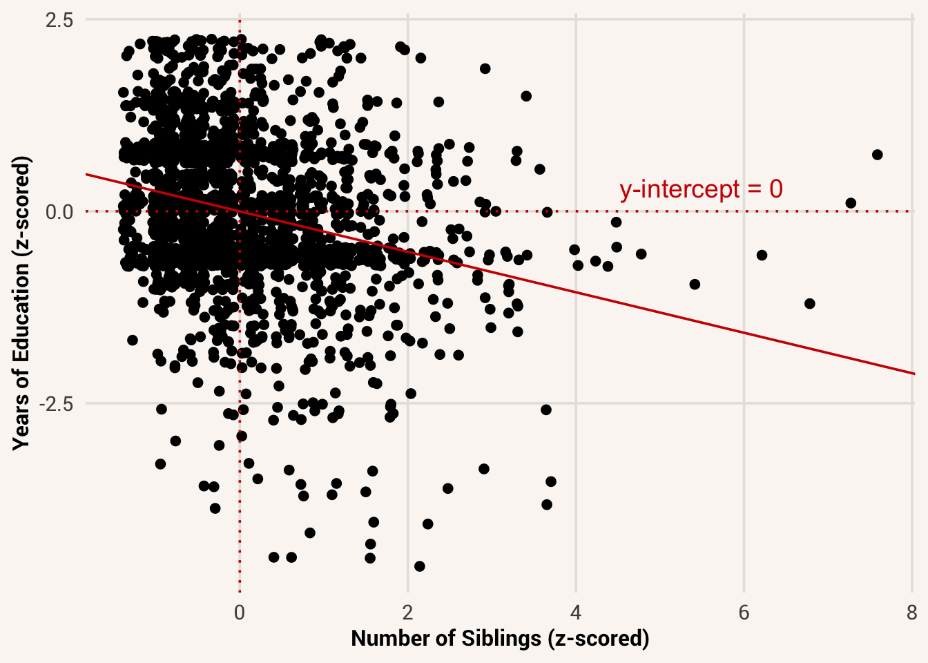
This standardized effect has the same value and same meaning no matter what the original units of the variables were. If we had measured education in months instead of years, the standardized effect would still be -0.26SD decrease in $Y$ per 1SD increase in $X$. The range of values measured in months would be larger, but so too would the standard deviation, so the z-scored values are the same. This makes it easier to compare effects across different studies and populations, and to interpret the size of the effect from the number alone.

In fact, this standardized coefficient is something we’ve seen before! If we were to calculate the Pearson correlation between highest_year_of_school_completed and number_of_brothers_and_sisters, we would get:

This reveals a deeper understanding of what the correlation calculation is doing: it is finding how much the mean of $Y|X$ changes as a linear function of $X$, in standardized units. This also means that we can interpret standardized model coefficients like a correlation, with the sign indicating the effect direction and the size (from -1 to 1) indicating the effect strength.

Note

Sometimes in research articles, scientists will use $b_1$ to refer to an unstandardized coefficient and $\beta_1$ for a standardized one, but this isn’t a rule and not always done. That’s probably what $b_1$ means though, if you see it when reading research.

10.5.2 Standardized model coefficients with a categorical explanatory variable

We saw in Chapter 6 that the same correlation math works on interval and dummy-coded binary variables. Thus, if our model consists of a categorical explanatory variable, we can also z-score this type of variable to get a standardized $\beta_1$ value. In this case, the coefficient will be the same as the point-biserial correlation between $X$ and $Y$.

However, standardizing in this way can make things more complicated to interpret for a categorical explanatory variable. The effect size would be comparable with different studies that use different scales of measurement, but directly interpreting this effect as a change in $X$ that is any value other than 1 would be making predictions with values that aren’t possible for the categorical $X$ variable to have.

Because of this⁶, it is more common to use a different approach for standardizing the coefficient of a model with a categorical explanatory variable. Instead of z-scoring both variables, we simply divide the $\beta_1$ coefficient by the model’s $\sigma$ estimate:

\[\beta_1^{std} = \frac{\beta_1}{\sigma}\]

Since the interpretation of $\beta_1$ for a categorical explanatory variable is the difference in the mean of $Y|X$ between two groups, dividing the estimate by $\sigma$ lets us express how big this mean difference is relative to the variation within the groups:

\[\beta_1^{std} = \frac{\mu_{Y|X=0} - \mu_{Y|X=1}}{\sigma}\]

This standardized mean difference metric is also known as Cohen’s d.

Cohen’s d = a metric of standardized mean difference between two groups, calculated as the difference in group means divided by the pooled standard deviation of the two groups

10.6 Chapter summary

10.6.1 Learning goals

After reading this chapter, you should be able to:

Explain what the best fitting line is in the context of an association between variables
Write the General Linear Model (GLM) equation form
Fit a statistical model using a GLM with an interval or categorical explanatory variable
Interpret the meaning of the GLM coefficients in the context of interval and categorical explanatory variables
Find and interpret standardized versions of GLM coefficients

10.6.2 New concepts

overfitting: When a model fits the training data too closely and fails to generalize to new data.
General Linear Model: a statistical model where the prediction equation takes the form of a linear equation.
effect: the magnitude of change in the target variable parameter associated with a one-unit change in the explanatory variable.
reference group: the category of a categorical explanatory variable that is assigned a value of 0 when dummy coding, and to which other groups are compared.
standardized coefficient: a statistical model coefficient that has been transformed to be in terms of standard deviations of the variables rather than their original units.
Cohen’s d: a metric of standardized mean difference between two groups, calculated as the difference in group means divided by the pooled standard deviation of the two groups.

10.6.3 New R functionality

predict()

It is also commonly called a regression model↩︎
More precisely, it’s an equation where the coefficients are multiplicative weights applied to explanatory values that are added together; the weight applied to an explanatory variable is the same no matter the value of that variable and different variables make separate contributions↩︎
“Effect” sounds like we’re implying that $X$ causes $Y$ in some way, but remember that models of the data generation process can encode both our ideas about real causes as well as our ideas about what information causes our guesses about another variable, even if those variables aren’t directly causing each other in the real world. Just because a model suggests an effect of $X$ in the statistical sense doesn’t mean changing $X$ would directly impact $Y$ in reality. It only affects what we predict about $Y$’s values.↩︎
If that doesn’t seem accurate, maybe there’s other important explanatory information missing from our model? ?sec-ch12 explains how to add multiple explanatory variables↩︎
Both the “education ~ siblings” model and the “education ~ sex” model fit the data pretty well - this illustrates how a dataset could come about through multiple processes. A good fit for your hypothesized model thus doesn’t mean your idea is the one definite data generation process in the real world.↩︎
And other reasons, like the fact that point-biserial correlations approach 0 when the distribution of $X$ is highly imbalanced even when the strength of association with $Y$ doesn’t change, since the variance of a binary $X$ approaches 0 as proportion $p$ decreases. See this paper for more mathematical detail.↩︎