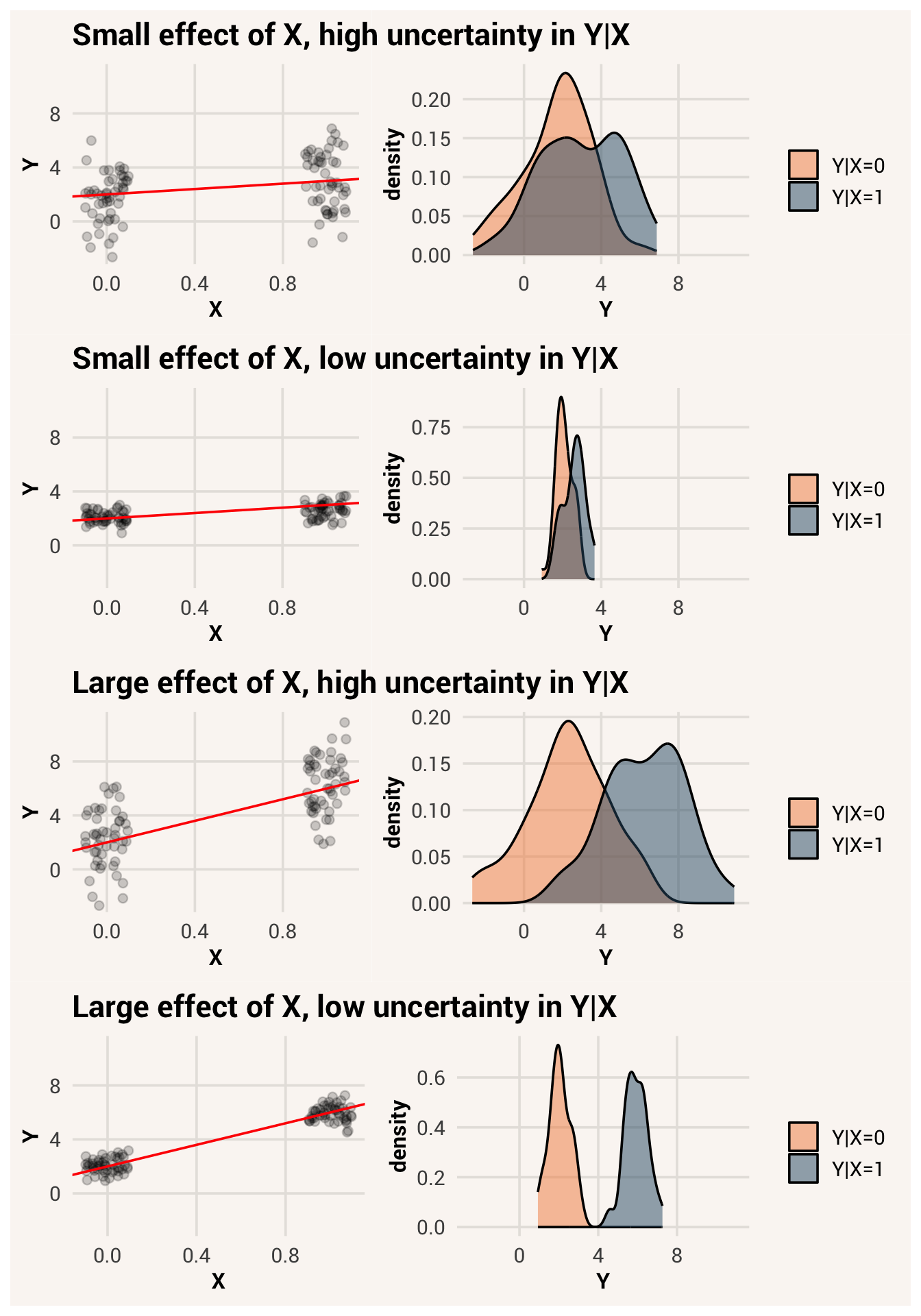
11 Interpreting Model Uncertainty

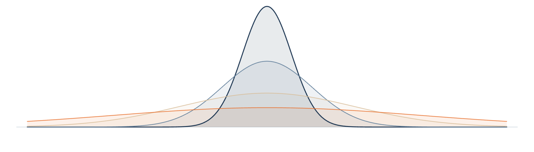
Last chapter we interpreted the $\beta$ coefficients in the prediction equation of a statistical model and evaluated what they mean about the role of an explanatory variable in a data generation process. This is useful information both for explanation research goals (e.g. “does $X$ influence $Y$?”) and for prediction goals (e.g. “what is the most likely value of $Y$ given what we know about $X$?”).

Stopping our model interpretation here, however, can leave us with an incomplete understanding. Seeing a big number for $\beta$ might make us think that $X$ is the most important variable for explaining $Y$, when this model of the data generation process could actually be critically incomplete and there is still uncertainty in $Y$ that would be explained better with other information. Similarly, making a prediction for some value of $Y$ given $X$ doesn’t tell us how good that guess is - how far off will we be when we make such a prediction?

In order to have a more complete understanding of our statistical model’s performance, we also need to interpret the other value that the model fitting procedure gives us: $\sigma$, in the observation model $Y_i \sim N(\mu_i, \sigma)$. In this chapter we will cover this interpretation step.

11.1 Prediction accuracy

Sometimes in a prediction goal, we want to predict a summary statistic of a large group of data. This is useful to do when our research is about group-level attributes, like overall student graduation rate under different financial aid strategies or the average number of customer service calls to expect at different times of day.

However, other times your goal is to make predictions about individual observations. In this case the estimand is not a summary statistic of a group, such as $\mu_i$, but how well you can predict the value of the target variable for specific observations $y_i$ when $X=x_i$.

We face some difficulty in doing this when we’re dealing with a probabilistic data generation process. Recall that in this sort of process, we can’t perfectly predict specific data values, only their probability of happening. For instance, here is a plot of the distribution of highest_year_of_school_completed values in the GSS dataset for people who have 4 siblings specifically:

Despite having the same value on the explanatory variable, these people still vary in their education attainment. So what do we do if we need to guess one specific value to accomplish our research goal?

If we don’t know someone’s $y_i$ value, but we do know their $x_i$ value and we have a best-fitting statistical model that tells us $P(Y|X)$, we could go with whatever value of $Y$ is most likely to happen when $X=x_i$. We will call this guess we make for the target value $\hat{Y}$ (“Y hat”) to distinguish it from real $Y_i$ values.

In the model we’ve been working with the last couple chapters, $Y_i \sim \mathcal{N}(\mu_i, \sigma)$ and $\mu_i = \beta_0 + \beta_1X_i$, we are assuming the data generation process creates normally-distributed target data, and the mean of these conditional distributions is influenced by $X_i$. This is a really common model form to use, and is altogether known as doing ordinary least-squares (OLS) regression, for a reason we will understand shortly. If we are correct that the observation model is a normal distribution - that $X$ influences what the central score is and observations are randomly and normally distributed around that - then the most likely value to happen, and the one we should use for $\hat{Y}$, is the mean of the distribution $\mu$. So we can use our model to tell us the most likely value of $Y$ given $X$ by calculating $\hat{Y_i} = \mu_i = \beta_0 + \beta_1X_i$.¹

ordinary least-squares (OLS) regression (OLS regression) = a statistical model that assumes the conditional probability distribution of target variable is normally distributed and the mean of that distribution is a linear function of the explanatory variable(s); under these assumptions, the best-fitting coefficients are those that minimize the sum of squared residuals

Here is the predicted $\hat{Y}$ value for people with $X=4$, drawn as a red line on the previous histogram:

Even though 13.62 is the most likely value in this conditional probability distribution, if we had guessed this value as the years of education for everyone with 4 siblings, clearly we’d be wrong most of the time². Written mathematically, $Y_i - \hat{Y_i} \neq 0$. We’d be less wrong on average than if we had guessed any other single number since this is the most likely value of the normal conditional probability distribution, but we’re still wrong because there is a difference between the $\hat{Y_i}$ prediction we made and the true value $Y_i$ for each person. This is known as the prediction error or residual for that person under our current statistical model. It is often denoted as $\epsilon$, such that:

residual = the difference between what a statistical model predicts for an individual observation and the observation’s true value.

\[\epsilon_i = Y_i - \hat{Y_i} \tag{11.1}\]

Since we’re using $\mu_i$ as the value for $\hat{Y_i}$, the residual in the case of out model is how far someone’s target value is from the mean of the conditional probability distribution expected for everyone with certain explanatory variable values.

How big is our prediction error / residual for each person? We can again make a plot, but this time we’ll plot the difference between $\hat{y_i}$ and $y_i$.

The shape of the histogram didn’t change, but the values on the x-axis did. Now, we are looking at the difference between a guess $\hat{y_i}$ and each real data point. Think of these residual values as how much our guess missed by.

Now let’s plot the residuals for every data point in this data set, not just the people with 4 siblings. We can find these quickly with the function resid(), where the argument is the model object.

Exercise

Use resid() to calculate the residuals for every data point in model and store them in a new dataset column called residuals.

We can think of each residual as a prediction error. We used a different value for $\hat{y}_i$ for each person depending on what their $x_i$ value is and what the prediction equation $\beta_0 + \beta_1x_i$ calculated, but we can still compute $y_i - \hat{y}_i$ for everyone and thus get a residual value. The distribution of all of them together is called the error distribution or residual distribution.

residual distribution = the distribution of residuals from a statistical model; also known as the error distribution

11.2 Quantifying prediction accuracy

If prediction for individual observations is our goal, we would like to quantify how good our model is for making predictions about all people. In other words, it would be useful to summarize this whole residual distribution. We can lean on the distribution summary metrics we already know to do this.

Recall when we first learned about spread metrics in Chapter 5. We first saw that trying to quantify spread as simply the sum of all deviations from a central value didn’t work, because some values were negative and positive and they canceled each other out. Because model residuals can also be positive or negative (we can guess too low or too high), this same reality applies:

Instead, if we make sure all deviation values are positive by squaring them, we can calculate the sum of squares. Specifically, when talking about residuals, we can sum up the squared residuals since a residual is a deviation score between a predicted value and a true value. This metric, when talking about model residuals, is called the residual sum of squares or sum of squared errors (SSE).

sum of squared errors (SSE) = sum of squares calculated for a model’s residual distribution; also known as the residual sum of squares

\[SSE = \sum_{i=1}^{n} (Y_i - \hat{Y}_i)^2 \tag{11.2}\]

Exercise

Calculate the sum of squared errors for the predictions model makes.

Reveal answer

sse <- sum(gss_clean$residuals^2)

Because sum of squared errors is just the sum of squares equation applied to a distribution of residuals, the same interpretation applies to this value as we would make with any other sum of squares. For the same amount of data, a larger value means more spread in the residual distribution. More spread in the residuals means there are more large residuals relative to small ones - our model is worse at predicting individual data points.

Here’s the sum of squared error calculated for the model predicting education using respondent sex. Which model do you think would make more accurate predictions - the one above using number of siblings, or using sex?

The reason ordinary least squares regression - a statistical model with the general linear prediction equation form and normal observation model family - has its name, is because under these assumptions the optimal coefficient values in the model are the ones that make a line that minimizes the sum of squared errors; making the data points “regress” towards the line of best fit as much as possible.

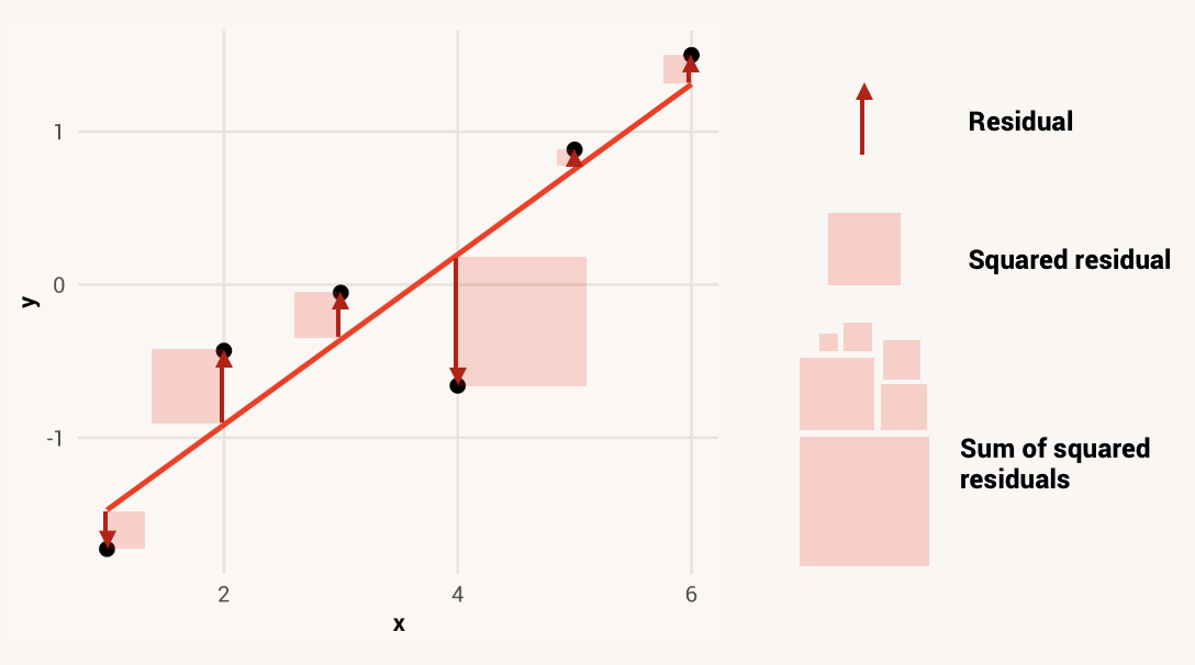
Figure 11.1: Visualization of where the magnitudes come from for residuals vs. squared residual vs. sum of the squared residuals (sum of squared error).

However, a larger SSE value can also occur just because there are more data points. So we can also calculate the typical amount of squared error per observation, called the mean squared error (MSE). This is similar to calculating the variance of the error distribution, except instead of dividing by $n-1$, we divide by $n-k-1$ where $k$ is the number of explanatory variables in the prediction equation³.

mean squared error (MSE) = variance of the residual distribution

\[MSE = \frac{\sum_{i=1}^{n} (Y_i - \hat{Y}_i)^2}{n-k-1} \tag{11.3}\]

Finally, because MSE is in units of squared residuals, it is tough to concretely interpret by how much our guesses are typically wrong. So we can take the square root of MSE to get back to the original units of the target variable. This is called the residual standard error (RSE), and is like calculating the standard deviation of the residual distribution:

residual standard error (RSE) = expected standard deviation of the residual distribution from a model

\[RSE = \sqrt{\frac{\sum_{i=1}^{n} (Y_i - \hat{Y}_i)^2}{n-k-1}} \tag{11.4}\]

When we first learned about standard deviation, we learned that the straightforward interpretation of it is the typical amount of deviation from the mean within a data distribution - if someone guessed the mean value for every data point, on average they would be off by plus or minus the standard deviation amount. We can interpret the RSE of the residual distribution the same way. It is the typical amount of prediction error our statistical model makes when predicting individual data points.

11.3 Prediction error as uncertainty

Now let’s look back at what our model fitting procedure identified as the $\sigma$ parameter for the normal observation model:

Look familiar? This is the same value as the RSE we just calculated from the residuals.

We know from earlier chapters that $\sigma$ is the spread parameter for a normal probability distribution. Because RSE and our model’s estimate of $\sigma$ are the same value, we can also interpret RSE as the spread in the conditional probability distribution $Y|X$ - how much uncertainty there is in $Y|X$ after taking into account the explanatory variable⁴.

It makes sense that a bigger spread in the conditional probability distribution would mean we have worse prediction error when making individual guesses - there are more likely options to choose, and thus more room for being wrong. But it also means RSE / $\sigma$ is relevant to us even if we don’t care about making predictions for individual observations. If we care about the whole probability distribution of $Y|X$, $\sigma$ is a piece of characterizing that. Finding that $X$ is associated with $Y$ means that not only does the conditional probability distribution $Y|X$ change location, it also narrows.

Figure 11.2: Visualization of the spread still in Y|X for a model with a lot of uncertainty / poor prediction accuracy, vs. a model with low uncertainty / good prediction accuracy.

11.4 The null model

We now know what $\sigma$ / RSE means about our model, so let’s practice interpreting the actual value from this example: 2.87. This is in units of years of education, so this value means that using the prediction equation output to make a guess for each observation will result in a missed guess by about 2.87 years on average. Alternatively, it means that the conditional distribution $Y|X$ from our model has a standard deviation of 2.87 years.

Is this a good prediction performance, or bad? The answer is probably relative to what your goals are, and whether a miscalculation of 2-3 years will still be useful information or not.

Or, we can judge our model by how much our prediction accuracy improves relative to some other method of guessing. In other words, even if we can’t predict the target variable perfectly, can we at least do better than random guessing by taking into account the explanatory variable?

Imagine we had to predict someone’s education attainment, but we had no other information about them. In that case, all we can do is use the central tendency of all $Y$ values as our best guess for each person. In this specific example, we would calculate our prediction as $\hat{Y} = \mu_Y = 13.74$, since 13.74 is the mean of all highest_year_of_school_completed values.

$\mu_i = 13.74$ is still a prediction equation, albeit a simple one without any explanatory variables and $\mu$ never varies. When we make a prediction/calculate an output parameter for the target variable without taking into account any explanatory variables, we are using what’s called the null model. Formally notated, the equations of the null model are:

null model = a statistical model that makes the same prediction about the target variable for every observation, with no inputs from any explanatory variables

\[Y_i \sim N(\mu, \sigma)\]

\[\mu = \beta_0 \tag{11.5}\]

This means $\beta_0$ in the null model can be understood as the mean of all $Y$ values.

We can actually visualize the null model with a line, like we did the linear model equation with an explanatory variable and line of best fit. It would just be a flat line with a y-intercept of 13.74, effectively making the same prediction for $\mu_Y$ at every level of some $X$.

We can fit this null model to find the best estimate of $\beta_0$ using lm(), except this time since there is no explanatory variable to include, we put NULL on the right side of the formula instead of the name of any explanatory variable.

In Chapter 10, we said $\beta_0$ was interpreted as the conditional mean of $Y$ when $X=0$. Here there is no $X$ variable in the model, so that second part of the statement wouldn’t make sense. But we still use $\beta_0$ to generate predictions for $Y$. Just in this case, it’s the mean value for all observations, i.e. the marginal mean of $Y$. For this reason, the null model is also sometimes called the intercept-only model.

11.5 Prediction improvement over the null model

Now that we have a null model, let’s interpret what its $\sigma$ value is:

This number means that, under the null model, the standard deviation of the marginal target probability distribution is 2.97. In other words, we would be wrong by 2.97 years on average if we used the null model to guide our predictions for target observations. Compare that to the 2.87 $\sigma$ value we got from the model with number_of_brothers_and_sisters as an explanatory variable. 2.87 is less than 2.97, which means taking into account number_of_brothers_and_sisters improves our predictions about the target variable.

To quantify this difference, we first need to calculate the sum of squares of the null model’s error distribution. We will call this the total sum of squares (SSTotal), since it is the total amount of variation in the target variable before taking into account any explanatory variables.

total sum of squares = the total amount of variation in the target variable before taking into account any explanatory variables

Now, if we subtracted the sum of squared errors of our model with number_of_brothers_and_sisters from the total sum of squares, we calculate the difference between these amounts:

The only difference between the null model and the original one we’ve been working with (we’ll call it the “full model” for contrast) is that the full model has an explanatory variable in it, while the null model doesn’t. Thus, the difference between SSTotal and SSE is the amount of target variation that the explanatory variable is able to explain away. This is called the model sum of squares (SSModel).

model sum of squares = the amount of variation in the target variable that the explanatory variable is able to explain

\[SSModel = SSTotal - SSError \tag{11.6}\]

Alternatively, we can think about prediction improvement as a percentage of the marginal variation. This is called the coefficient of determination ($R^2$ for short), and is defined as:

coefficient of determination ($R^2$) = the proportion of variation in the target variable that is explained by the explanatory variable(s)

\[R^2 = \frac{SSModel}{SSTotal} = \frac{SSTotal - SSError}{SSTotal} \tag{11.7}\]

You might also see $R^2$ written as:

\[R^2 = 1 - \frac{SSError}{SSTotal}\]

which is equivalent. $\frac{SSError}{SSTotal}$ is the proportion of original error that is still present in our predictions once we take $X$ into account. If SSE is very small relative to SSTotal, that means $X$ has explained away most variance.

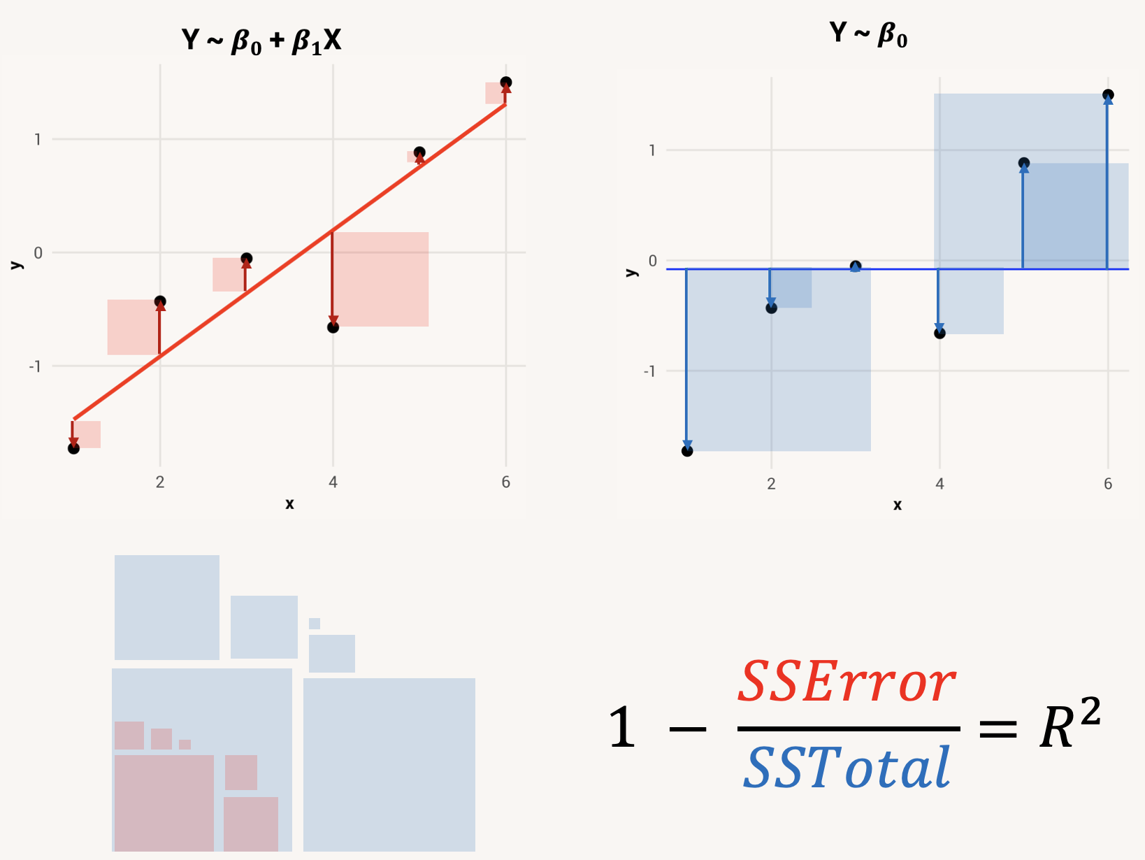
Figure 11.3: Visualization of the relative magnitudes of sum of squared errors in the prediction model fitted with an explanatory variable (red; SSError) vs. the null model (blue; SSTotal).

$R^2$ is a proportion, so its value is always between 0 and 1. We should interpret this value as the percentage of variation in the target variable that the prediction equation can explain away. If our model’s $R^2$ value is near 0, that means the explanatory variable doesn’t really help us make better predictions about the target variable. It explains very little variation in the target. The closer our $R^2$ gets to 1, the closer we are to explaining away all the variation in the target.

Or, thinking about $R^2$ in terms of spread in the the marginal and conditional probability distributions of $Y$, it is how much narrower $Y|X$ is when we include an explanatory variable vs. when we don’t. Still another way to write the equation for $R^2$ is thus:

\[R^2 = 1 - \frac{Var(Y|X)}{Var(Y)}\] The greater the $R^2$ value, the less uncertainty is left in the target variable after taking into account the explanatory variable. If we somehow came up with a model that produced an $R^2$ of 1, that would mean there would be no uncertainty in the target variable after taking into account the explanatory variables; we could predict the target variable perfectly and would have a deterministic data generation process.

Let’s calculate the $R^2$ for our model object, by finding the ratio of SSE and SSTotal and subtracted from 1:

Exercise

Calculate $R^2$ using the equation \[R^2 = 1 - \frac{SSError}{SSTotal}\] Remember that we saved SSE as sse and SSTotal as sst.

We can also access this value about our model a quicker way. When we save the output of an lm() call to an object, typing that object name gives us info about what model formula we fit and the best-fitting values for the prediction equation coefficients. But if we use the function summary() with our model object as an argument, we get a lot more info about it:

There is some information here we don’t understand yet (don’t worry, we’ll get to it all by the end of the book!), but for now focus on the following sections:

Residuals: this is a summary of the residual distribution. It’s as if we calculated summary statistics on gss_clean$residuals.
Residual standard error: this is the RSE value we calculated, and is the same as the $\sigma$ parameter in the observation model. There’s a mention of “2338 degrees of freedom”, which is the name of the $n-k-1$ denominator used for calculating MSE and RSE.
Multiple R-squared: this is the $R^2$ value we calculated by hand; the proportion of variation in the target variable that is explained away by the explanatory variable. “Multiple” is used because $R^2$ can also be calculated for a model with multiple explanatory variables. We’ll see that in action next chapter.

To get any of these values individually, something good to know is that the output of summary(model) can itself be saved to an object, and that object will have all these values as properties. We can access each of these properties with $ in the same way we access individual variables in a data frame. Here are all the properties of the model summary:

There are many properties in here that we previously used a function or hand calculation to produce: residuals, coefficients, sigma, and r.squared.

Exercise

Use the $ operator to output to the console just the r.squared property of model_summary.

Optional: going deeper

If you noticed that $R^2$ is using the same letter as correlation $r$, that is because $R^2$ for an OLS model is mathematically the square of the Pearson correlation between what the model predicts for the target values and what the values actually are.

To see how this works, first remember the definition of a residual we wrote in Equation 11.1:

\[\epsilon = Y - \hat{Y}\]

Rearranging this equation:

\[ Y = \hat{Y} + \epsilon\]

The covariance of $Y$ and $\hat{Y}$ is:

\[ Cov(Y, \hat{Y}) = Cov(\hat{Y} + \epsilon, \hat{Y}) = Cov(\hat{Y}, \hat{Y}) + Cov(\epsilon, \hat{Y})\]

When using a normal distribution for an observation model as we have, we assume the same $\sigma$ parameter regardless of the value of $X$. This means $Cov(\epsilon, X) = 0$. Since $\hat{Y}$ is a linear transformation of $X$, this also implies $Cov(\epsilon, \hat{Y}) = 0$ and drops out of the equation. Thus,

\[Cov(Y, \hat{Y}) = Cov(\hat{Y}, \hat{Y}) = Var(\hat{Y})\]

Now, recall the formula for Pearson correlation:

\[Cor(Y, \hat{Y}) = \frac{Cov(Y, \hat{Y})}{sd(Y)sd(\hat{Y})} = \frac{Var(\hat{Y})}{sd(Y)sd(\hat{Y})}\]

Since $Var(\hat{Y}) = sd(\hat{Y})^2$, we can simplify this to:

\[Cor(Y, \hat{Y}) = \frac{sd(\hat{Y})}{sd(Y)}\]

Squaring both sides gives us:

\[Cor(Y, \hat{Y})^2 = \frac{Var(\hat{Y})}{Var(Y)}\]

Which is just a different way of writing:

\[r^2 = \frac{\frac{SS_\hat{Y}}{n-1}}{\frac{SS_Y}{n-1}} = \frac{\frac{SSModel}{n-1}}{\frac{SSTotal}{n-1}} = \frac{SSModel}{SSTotal}\]

11.6 Sources of uncertainty

Besides just quantifying uncertainty in our models, it’s good to think about why there is uncertainty in the first place, and where it comes from. We know we are modeling probabilistic processes, which means different things can happen even with the same inputs; we are unlikely to ever be able to perfectly predict data about humans and explain away all the uncertainty. But it’s important to remember why that is.

11.6.1 Missing parts of the data generation process

In a simple model like the one we’ve been working with - just one explanatory variable in a linear form - it’s unlikely that we have captured all the pieces of information that explain the target variable. For instance, imagine you are a clinical psychology researcher trying to understand what causes debilitating depression. One reason could be a significant stressor like losing a loved one. But there are many people who bounce back fairly healthy after such a stressor, while there are many people with depression who have not had such an experience. People are multifaceted and complicated, so just knowing this one piece of information about somebody doesn’t resolve all the uncertainty about whether they will develop depression. Modeling depression as the product of just one input means we’re probably missing fundamental pieces of the data generation process.

If we did know what else can cause depression, we could include that information in our model as well. Perhaps a significant stressor increases the risk of depression, but so do things like genetics, social connection, or neuroticism. By taking all that information into consideration, rather than making decisions based on just one explanatory variable, we could explain additional variance in depression and make better predictions. In the next chapter we will discuss how to make and interpret statistical models with multiple inputs.

11.6.2 Incorrect model form

The wrong form of a statistical model can also lead to prediction errors. For instance, if we know that a significant stressor increases the risk of depression, but only up to a certain point, then a linear model will not capture that reality. A linear model assumes that each unit increase in the explanatory variable has the same effect on the target variable, but if the relationship between stress and depression is more like a threshold than an increasing rate, a linear model will overestimate the effect of stressors above that threshold and underestimate the effect of stressors below it.

If we do the model fit checking we are supposed to do by simulating plausible data with our model and comparing it to the distribution of real data, we would see this issue due to the fact that the simulated data would have a different distribution than the real data. But if we ignored this step and tried to use a misspecified statistical model to make predictions, we would poorly predict the target variable in certain ranges of the explanatory variable, and we would consistently make these missed predictions for everyone with those values of the explanatory variable. This is more insidious than random prediction errors. If we are wrong when making predictions for new data, and we are systematically wrong in a certain direction rather than randomly guessing too high or too low, that suggests we have an incorrect idea about the form of the data generation process.

11.6.3 Measurement error

Even if we correctly identify all important pieces of a data generation process and use the right model form, we can still have uncertainty and prediction error in the target variable because of the way we measured those pieces.

Consider our depression research again - how do we measure someone’s depression level? If you’re like many other researchers, you might think a series of questions about depression symptoms is a good idea: “In the last week I: 1) felt sad (1-7); 2) had little interest in activities (1-7); 3) felt worthless (1-7)”, etc. People with and without depression probably answer these questions differently on average, but responses to these questions aren’t perfect measurements of depression because they are subjective and possibly produced by other things too. These measured survey values are related to the true, latent depression values, but they’re not exactly the same.

Statistical model uncertainty can come from an incomplete understanding of what predicts depression, but also imprecision in how well latent constructs map onto the measurements we have. The less well our measurements reflect the true target or explanatory variable of interest - i.e. the more measurement error there is - the more uncertainty will remain in our model even if it captures the correct data generation mechanism for the latent construct.

A class of statistical models known as measurement models are designed to acknowledge this reality and explicitly model ideas of the data generation process between latent and measured values. Things we’ve talked about before concerning measurement error, like assuming that the error is random and repeated measures of the same thing will vary evenly around the true value, are examples of assumptions from a measurement model called classical test theory. In this case, such an assumption would be encoded as an observation model like $Y_{measured} \sim \mathcal{N}(Y_{true}, \sigma)$ where $\sigma$ is magnitude of measurement error. If you’ve heard of analysis tools like factor analysis, item response theory, or structural equation modeling, these are all examples of approaches to measurement modeling.

These ideas of latent vs. measured variables in psychology are a big reason why this book takes the statistical modeling approach that it does for teaching about data analysis. You can think about the prediction equation as your idea about how the latent construct comes about, while the observation model is your idea about how the measurements come about. The two together are your full idea of a data generation process of behavior, physiology, and self report that arise through latent psychological processes⁵.

11.7 Different model pieces as different estimands

At this point, let’s take stock of what we know about statistical models so far. We know that models are how we quantify our ideas of a data generation process so that we can fit them, simulate from them, and test them against real data. We know how to write equations that encode the four components of a data generation process, and we know how to interpret the numbers in those equations.

Each of these numbers - the coefficients of the prediction equation, the parameters of the observation model, predictions that the model makes - are all quantities about the data generation process we might have hypotheses about. Thus, each of these are estimates of different estimands. Below is a table of some example estimands we might be interested in as researchers, and the part of our statistical model that would give us the corresponding estimate.

Estimand	Estimate in statistical model
Typical $Y$ scores	$\beta_0$ in null model
Variation of $Y$ scores	$\sigma$ in null model
How much $X$ shifts predictions of $Y$	$\beta_1$ in full model
Uncertainty in $Y\|X$ probability distribution	$\sigma$ in full model
How much variation in $Y$ is explained by $X$	$R^2$
Predicted $Y$ value for specific observations	$\hat{Y}$ for a given $X=x_i$
Prediction accuracy of individual observations	RSE in full model

When we interpret one estimate from a model for what it means about the estimand we are interested in, it’s important to remember that this interpretation is only valid in the context of the rest of the model. E.g., the effect of number_of_brothers_and_sisters on highest_year_of_school_completed ($\beta_1$) is only -0.27 if we accept the assumptions that the form of the data generation process is linear, that the observation model is a normal distribution, and that there are no other important explanatory variables we are missing. If any of those assumptions are wrong, then our estimate of the effect may not be accurate for what the data generation process actually is. Building good scientific theory is hard work!

11.8 Chapter summary

11.8.1 Learning goals

After reading this chapter, you should be able to:

Make predictions for individual data points using a fitted statistical model
Quantify prediction accuracy for one data point and for the model overall
Define a null vs. full model
Quantify prediction accuracy for the full vs. null model
Explain sources of uncertainty in statistical models
Identify estimates of different estimands in a statistical model

11.8.2 New concepts

residual: The difference between what a statistical model predicts for an individual observation and the observation’s true value.
residual distribution: The distribution of residuals from a statistical model; also known as the error distribution.
sum of squared errors (SSE): Sum of squares calculated for a model’s residual distribution; also known as the residual sum of squares.
mean squared error (MSE): Variance of the residual distribution in a model.
residual standard error (RSE): Expected standard deviation of the residual distribution from a model.
null model: A statistical model that makes the same prediction about the target variable for every observation, with no inputs from any explanatory variables.
total sum of squares: The total amount of variation in the target variable before taking into account any explanatory variables.
model sum of squares: The amount of variation in the target variable that the explanatory variable is able to explain.
coefficient of determination ($R^2$): The proportion of variation in the target variable that is explained by the explanatory variable(s).

Note that using $\mu_i$ as the value for $\hat{Y_i}$ happens specifically in models with a normal observation model. If we thought our target’s probability distribution was some other family, we’d need another way to get the most likely value in the distribution.↩︎
Actually all of the time, since people only responded with whole numbers for years.↩︎
Chapter 15 will explain why we’re dividing by not quite $n$. Patience a little longer…↩︎
This $\sigma$ value is only a parameter for a normally-distributed conditional probability distribution, so it and its interpretation only apply to statistical models that use such an observation model. If you are working with a kind of target variable that is distributed differently and has different parameters, you would use different metrics to quantify prediction accuracy.↩︎
Building on this idea, using just a probability distribution as an observation model says we don’t know what specifically causes observations, just that they tend to cluster around a latent parameter. But you could have more elaborate observation model ideas, where there is another level of explanatory variables and equations that explain how an observation value comes about from a latent parameter. Multiple levels of equations like this are covered in ?sec-ch24.↩︎

Estimand	Estimate in statistical model
Typical \(Y\) scores	\(\beta_0\) in null model
Variation of \(Y\) scores	\(\sigma\) in null model
How much \(X\) shifts predictions of \(Y\)	\(\beta_1\) in full model
Uncertainty in \(Y\|X\) probability distribution	\(\sigma\) in full model
How much variation in \(Y\) is explained by \(X\)	\(R^2\)
Predicted \(Y\) value for specific observations	\(\hat{Y}\) for a given \(X=x_i\)
Prediction accuracy of individual observations	RSE in full model