16 Null Hypothesis Testing
Last chapter we discussed how to estimate the value of estimands in the population using data samples and estimators. We discussed biased and unbiased calculation of the estimate, interpreting its effect size magnitude, and interpreting the estimation precision. Following estimation procedures gives you information about what the value of the estimand is. Having an idea of this value then helps you make informed decisions.
Estimation is also helpful if you don’t have a starting idea about what the estimand will be. What percentage of people will have side effects from a drug? How accurately can we predict students’ college performance from aptitude tests? What is the role of social media in influencing political polarization? If you start out with these questions but not a good idea about an answer, collecting some data, fitting statistical models or other estimators, and then interpreting the estimates can give you a better idea of the quantity of interest (and an idea of confident you can be in that estimate).
However, sometimes you do start out with an idea of what the estimand’s value is. This would be the case if you have scientific theories about data generation processes. In this case, the point of collecting data is to see if reality is congruent with your expectations or not. If you have pre-existing expectations for what your data will show, that is called having a hypothesis. The process of testing how well data correspond with a hypothesis is another inference process is called hypothesis testing. In this chapter, we will discuss how to do this.
hypothesis testing = the process of comparing real data to hypothesized expectations as a way of deciding whether the expectations were good or not.
16.1 Specifying a hypothesis
In order to perform hypothesis testing, we first need to specify a hypothesis. You may be used to doing this verbally, with a research question like “there will be a difference between the experiment groups” or “one variable will affect another.” But as we discussed when first learning about statistical models, these verbal statements are vague and could describe a lot of different outcomes. That means it is hard to test whether or not a hypothesis such as this is supported or refuted by data.
16.1.1 Specific estimands
Instead, a good hypothesis is focused on a specific estimand. That means before you can specify your hypothesis, you also need to specify your estimand.
For example, let’s come back to the dataset used in the previous chapter consisting of personality scores and life outcomes. If you say you are interested in personality and leadership behavior, does that mean you are interested in the effect of a personality variable on leadership, or are you more interested in overall how well can your personality model predict leadership behavior? Are you interested in how well the model predicts data for everyone, or are you interested in what specific prediction is made for observations with specific input values? The foci of all of these questions are different estimands we have discussed previously, such as \(\beta_0\), \(R^2\), or expected \(Y|X=x_i\).
It is also important to know what context you are assuming for your estimand. If you are interested in the effect of extraversion on leadership, is that effect in a model with only the extraversion variable included? Or are you specifically focused on the partial effect of extraversion over and above other explanations in a multivariable model? If so, what other possible explanations of leadership did you control for? It is important to write down and model your ideas about the overall data generation process because, even if you are only interested in investigating a piece of that process, the effect size of that piece might depend on other pieces.
16.1.2 Specific expectations
A good hypothesis is also a specific expectation about what the value of the estimand will be. In order to test your hypothesis against data, you can’t simply hypothesize “there will be a big effect of extraversion on leadership.” You need to state, numerically, what “big” means. Do you think the effect value will be at least 0.5, 1.5, -1.5? Do you think the prediction performance will be an \(R^2\) of 20%? 30? 42.8%?
16.2 Hypothesis testing
Once you have chosen a specific estimand for your hypothesis and provided a specific numeric expectation for the value of that estimand, only then can you test your hypothesis.
To do so, our knowledge of sampling distributions comes back to help. The essence of hypothesis testing is to 1) see what kind of estimates would be reasonable to expect given our hypothesized estimand value and sampling procedure, 2) calculate an estimate in our data, and 3) compare our estimate to the expected sampling distribution.
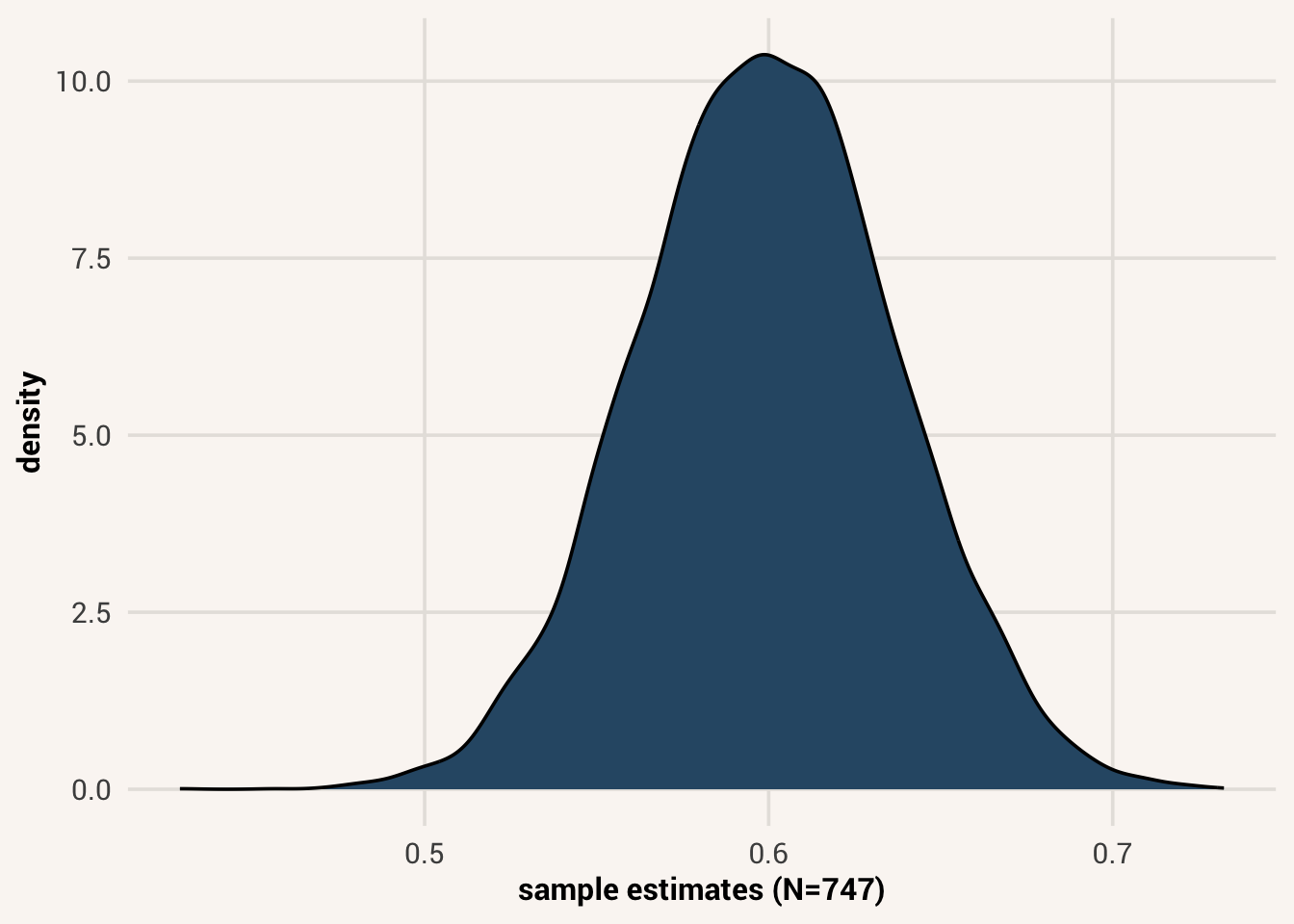
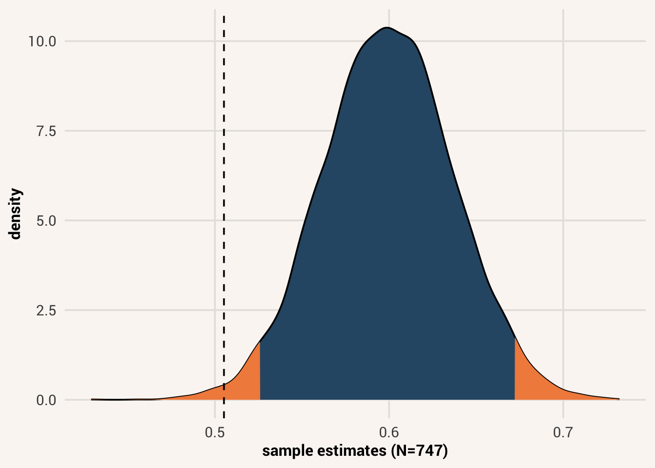
For instance, let’s say we are interested in the effect of extraversion on leadership (no other control variables), and we hypothesize that leadership scores will change by 0.6 for every 1-unit increase in extraversion (i.e., that \(\beta_1 = 0.6\)). If 0.6 was the true value of this estimand in the population, then we likely wouldn’t get exactly 0.6 as an estimate in a finite data sample. But the estimates we would get over repeated samples would cluster around 0.6, and on average would deviate from 0.6 by the standard error amount (which, in this specific case with a sample size of 747, is about 0.037). Figure 16.1 shows what this sampling distribution would look like visually.
Now, let’s actually calculate an estimate of the effect in real data by fitting a statistical model:
In our data, we estimate this effect to be about 0.51. Figure 16.2 shows how this value compares to the sampling distribution of our hypothesized value.
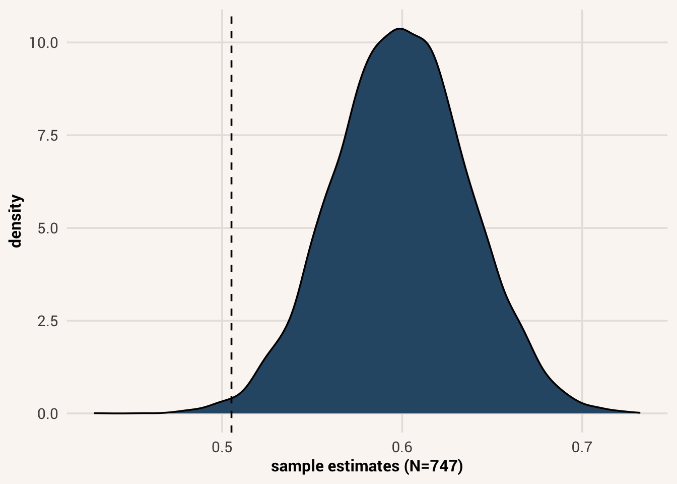
In a vacuum 0.51 might not seem like such a different number than 0.6; we may not consider those effect sizes to be meaningfully different. But in fact, given our sample size, it would surprising to get a 0.51 estimate if the true population effect were actually 0.6. It’s not impossible, but it’s in the tail extreme of the sampling distribution, making it very unusual to see.
It can be helpful to standardize estimates in the sampling distribution to see this better. Remember the equation for a z-score we first encountered in Chapter 5? There, we learned a z-score is calculated as \(z = \frac{x_i - \bar{x}}{s_x}\). A z-score helped us see where a data value was relative to the distribution of other values. We can bring that logic to our sample estimate here, finding out where an estimate of 0.51 would be relative to the sampling distribution. That version, when calculated for an estimate relative to its sampling distribution, is called a t-statistic.
t-statistic = standardization of an estimate relative to its sampling distribution, calculated as the difference between the estimate and sampling distribution mean divided by the estimated standard error.
\[t = \frac{\hat{\beta_1} - \beta_1}{\hat{SE_{\hat{\beta_1}}}}\]
To standardize our estimate of 0.51 as a t-statistic, we first find how far away it is from the hypothesized population value of 0.6 (0.09). Then, we divide that deviation by an estimate of the standard error1, 0.037. Solving this equation, we get a t-statistic of -2.58. An estimate of 0.51 is 2.58 standard deviations / standard errors below the sampling distribution mean.
We can also calculate how likely it would be to get an estimate like ours, or more extreme. That would be the probability of getting a sample estimate as far away, or farther, from the sampling distribution mean as 0.51 is. In other words, the probability of getting an estimate with a t-statistic in the sampling distribution of at least \(|t| = 2.58\).
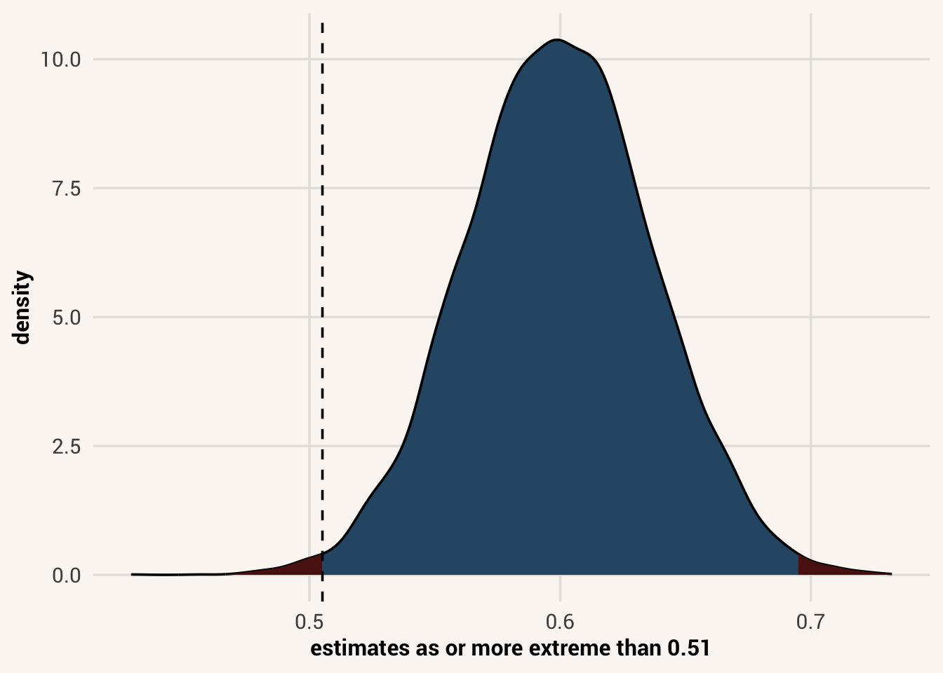
This probability is called the p-value of the estimate. More clearly, the definition of a p-value is the probability of getting an estimate as extreme or more extreme than the one we calculated, when the hypothesized population value is true. “Extreme” here means far away from the hypothesized population value - it could be extremely above, or extremely below. That’s why both tails in Figure 16.3 are highlighted2.
p-value = the probability of getting a sample estimate as extreme or more extreme than a calculated estimate, assuming the hypothesized population value is true.
In this situation, the p-value of a 0.51 \(\hat{\beta_1}\) estimate, assuming the true \(\beta_1\) is 0.6, would be 0.01. If 0.6 is the truth, only in 1% of random samples would we calculate an estimate as far away from 0.6 as 0.51 is, or farther.
16.3 Statistical significance
Now that we’ve seen this result, we have a decision to make. Do we think our hypothesized estimand value can reasonably create estimates like we observed in our data via our sampling process? Or is our 0.51 estimate so surprising that we don’t believe our hypothesis of 0.6 is the true state of the world?
Making this call is making a decision about an estimate’s statistical significance. If our calculated estimate is within the bounds of reasonable estimates to expect from our hypothesized population value, then that hypothesis is still on the table as a consideration for the truth. If our calculated estimate is very far away from the hypothesized value, such that it is extremely unlikely to be produced if the hypothesis were true, then we decide the estimate is statistically significant with respect to our hypothesized value and we reject the hypothesis. Something else is probably the truth instead.
statistical significance = a large enough difference between a hypothesized estimand value and one’s estimate that makes one reject the hypothesized value.
But what level of probability is needed to deem something statistically significant? There isn’t one correct answer to this, so most people use an arbitrary convention. Most commonly, they divide the sampling distribution into the 95% middle and the 2.5% high and low tail areas:
While not impossible, estimates in the orange parts of the curve are rather unlikely to happen if the hypothesis is true. Only 1 in 20 sample estimates would land in these areas. These areas also correspond to a p-value of 0.05 (5% probability of occurring). This cut-off level we use to make a decision of statistical significance is called the significance criterion, often abbreviated \(\alpha\) (“alpha”).
significance criterion \(\alpha\) = the level of probability used for making a decision of statistical significance about an estimate; if the probability of getting our estimate or more extreme is less than the significance criterion, significance is decided and the hypothesis rejected.
16.4 The null hypothesis
In practice, it can be quite challenging to come up with a specific numeric expectation for your estimand. This is especially true if your theory isn’t very mature yet. We may have ideas for verbal hypotheses right now (e.g., “there will be an effect of extraversion on leadership”), but not expectations about what specific number that vague idea translates to.
When you find yourself in this situation, one solution to start with is not to hypothesize a value that you expect to be the truth, but to hypothesize a value that you think is not the truth, or would be very uninteresting if it were. Then, if you reject that hypothesis, you’ve eliminated an uninteresting possibility.
For instance, rather than committing to a specific level of effect for extraversion right off the bat, we could pose a hypothesis that there is no effect of extraversion on leadership. In other words, our hypothesis is that \(\beta_1 = 0\). If we estimate an effect that is statistically significant with respect to a population value of 0, then we reject the hypothesis that there is no effect of extraversion. We still don’t know what exactly the effect is, and it might be a positive or negative effect. But we decided to eliminate the possibility that there isn’t an effect at all.
A hypothesis of no interest that you want to eliminate is called a null hypothesis. For shorthand, we write this specification as \(H_0\). Thus to say we are using a null hypothesis that \(\beta_1 = 0\), we’d write \(H_0: \beta_1 = 0\). Testing data against the null hypothesis is called null hypothesis significance testing (NHST for short).
null hypothesis = a hypothesis that the value of a population estimand is not a particular value.
Testing against a null hypothesis is common to do because it doesn’t require much effort or prior work from you to think of a specific estimand value that you actually expect. It eliminates an option for the population value instead of asking you to come up with a particular expectation.
16.4.1 Testing effect estimates
P-values of estimates with respect to a null hypothesis of 0 are the default in many statistical testing packages. For instance, if we just look at the summary output of a statistical model object:
We see a column “t value”. This is the t-statistic we discussed at the beginning of the chapter. In this case, because the statistic is 13.72, our estimate of 0.51 is about 13.72 standard errors above the mean of the sampling distribution when that mean is set to 0.
“Pr(>|t|)” is the next column. This is the p-value of that estimate for a null hypothesis \(H_0: \beta_1 = 0\). It is the probability of getting an estimate that is at least as far away from 0 as 0.51 is, when the true population value is 03. If we want to use a typical \(\alpha\) threshold of 0.05 for our significance criterion, then we can look at the “Pr(>|t|)” value on the extraversion estimate line and see if it is less than 0.05. Listed here is a very tiny p-value (<2e-16, needing scientific notation to write it!), so we decide to reject the null hypothesis that there is no effect of extraversion on leadership.
But now let’s consider a multivariable situation, where we hypothesize that conscientiousness is also an explanatory variable of leadership after controlling for extraversion.
TipExercise
Use the code block below to fit a linear model where Conscientiousness and Extraversion are the explanatory variables of Leadership. Use soto_work as the data frame.
We see estimates for both Extraversion and Conscientiousness here, as well as standard errors, t-values, and p-values. In this case the estimate for Extraversion has changed. That’s because we’re now modeling it in the context of conscientiousness, so the estimate is the partial effect of extraversion on leadership after controlling for conscientiousness. Likewise, the estimate for Conscientiousness is the partial effect of conscientiousness after controlling for extraversion.
Is extraversion a significant predictor of leadership, after controlling for conscientiousness? If we use a null hypothesis for this question, that would be saying \(H_0: \beta_{Extraversion} = 0\). In other words, since this is a null hypothesis, we want to eliminate the option of there being no additional effect of extraversion after considering conscientiousness. We don’t know what that partial effect would be, but we think it’s not 0 so we want that off the table.
The p-value for this estimate turns out to be <2e-16 again. It is extremely unlikely to get a partial effect estimate of 0.48 if the true population \(\beta\) were 0. Thus we reject this null hypothesis.
Do you think conscientiousness is similarly a significant predictor of leadership, after controlling for extraversion? In this case, the null hypothesis would be \(H_0: \beta_{Conscientiousness} = 0\) and our estimate of that is \(\hat{\beta} = 0.06\). However, the corresponding p-value is 0.136. This means there is a 13.6% chance of getting a partial effect estimate of 0.06 or more extreme if the true population \(\beta\) were 0. Since this is greater than our \(\alpha\) threshold of 0.05, we fail to reject the null hypothesis. Conscientiousness is not a significant predictor of leadership after controlling for extraversion.
Note the verbiage we just used when talking about conscientiousness. While we rejected the null hypothesis for extraversion, we failed to reject the null hypothesis for conscientiousness. Failing to reject the null hypothesis means that it is still a plausible candidate for the true population value.
Failing to reject a null hypothesis is not the same thing as accepting the null hypothesis. If we accepted the null hypothesis, that would mean we think the null hypothesis value is the one true population value. But we can’t know that with this approach. Null hypothesis testing can only help us eliminate options. If we fail to reject the null hypothesis, that means it is still a candidate for the truth, but so are a lot of other things! An estimate of 0.06 is plausible to get in a sampling distribution with \(\beta = 0\), but it is also plausible to get in a sampling distribution with \(\beta = 0.1\), \(\beta = 0.2\), \(\beta = 0.3\), etc. We can’t know which of those is the truth, so we can’t accept the null hypothesis as the truth.
In null hypothesis testing, we can only ever reject or fail to reject a null hypothesis. We can never accept it.
16.4.2 Testing model performance
While our discussion so far has focused on \(\hat{\beta}\) estimates in a model, we can also focus on different estimands and test those values against a null hypothesis. Which estimand to focus on, and thus which estimate to hypothesis test, depends on our research goals and should be decided up front before any analyses are done.
For instance, if we were not focused on the effect of a particular explanatory variable but instead on the predictive performance of a statistical model as a whole, our estimate of interest would be the model’s \(R^2\) value. The true \(R^2\) value in the population is the proportion of variation our specified model could explain if we had access to the entire population of data. Since we don’t, we can only calculate a \(\hat{R^2}\) estimate in our limited data sample. That’s the number we get in the summary() output:
Since this is an estimate, there is also a sampling distribution of \(\hat{R^2}\) values we could get if we drew repeated samples from the population. For instance, Figure 16.5 shows the sampling distribution of \(\hat{R^2}\) values we would get if the true \(R^2\) in the population were actually 0, and we estimated it over and over in samples of N=747.
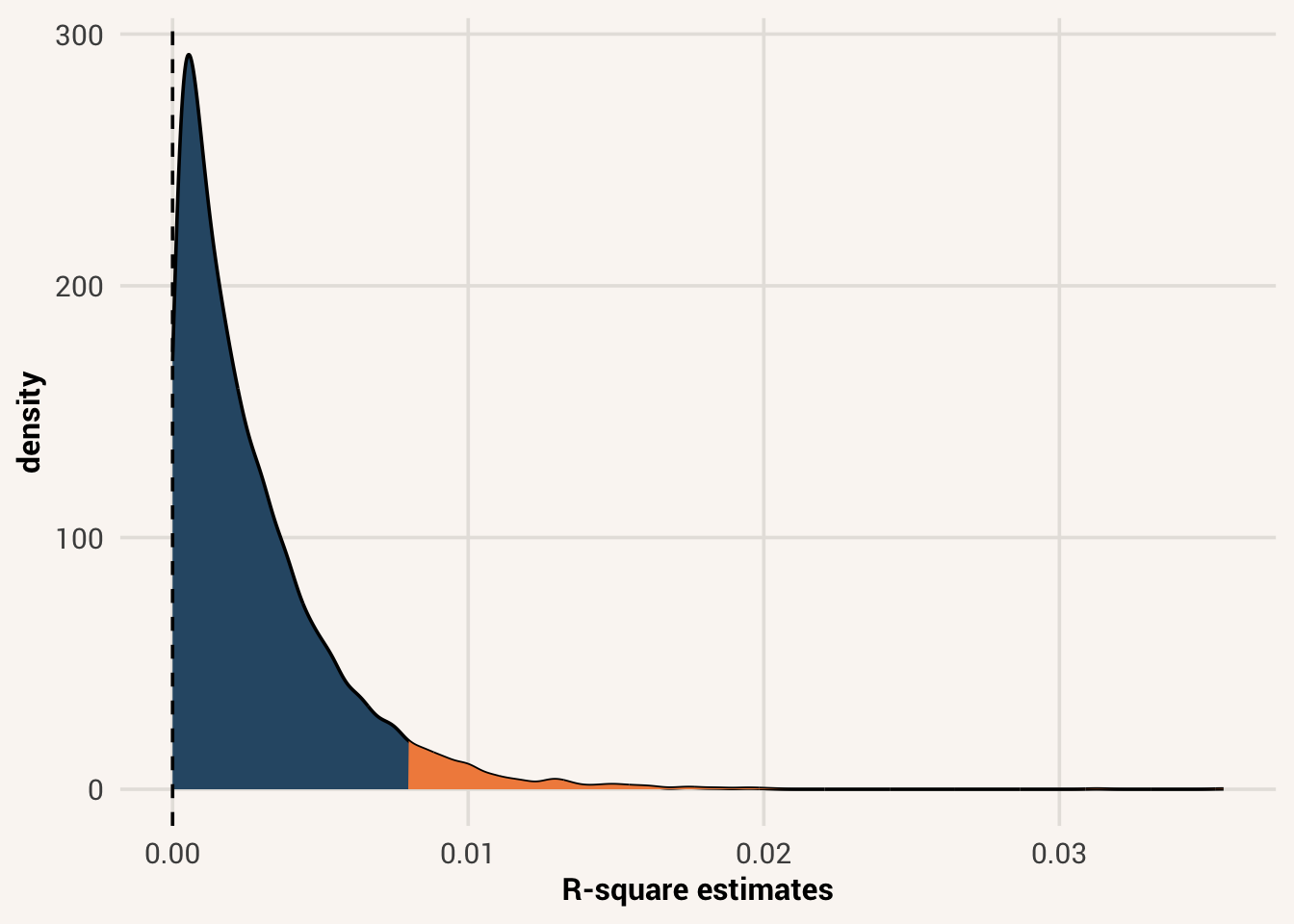
You’ll notice that this is shaped differently than the sampling distributions we previously saw. That’s because \(R^2\) is a proportion measure, with a lower bound of 0. Even if the true population \(R^2\) is 0, we can never get a \(\hat{R^2}\) estimate that is below 0 because of the way \(R^2\) is calculated. Instead, we can only get estimates that are 0 or higher, although much higher than 0 becomes increasingly less likely. This sort of distribution shape is called an F-distribution, named after the statistician Ronald Fisher who first described it.
F-distribution = a probability distribution of estimates that is bounded at 0 and has a long tail to the right.
The p-value of a \(\hat{R^2}\) estimate is thus the probability of getting an estimate as big or bigger than ours in a sample of N=747 when the true \(R^2\) is 0. To find that, look at the very last line that summary() returns, starting with “F-statistic”.
That line says the F-statistic is 95.46, which is the standardized value of our \(\hat{R^2|\) estimate in the F-distribution. There are 2 and 744 degrees of freedom, which means there are 2 explanatory variables (K=2) in the model and N-K-1 is 744 (N=747 - 2 - 1). Finally, the next value is the p-value of the whole model’s score: < 2.2e-16.
If we were testing against a null hypothesis \(H_0: R^2 = 0\) and using a significance threshold of \(\alpha=0.05\), would we reject the null hypothesis based on this p-value? What about if our significance threshold was more stringent, at \(\alpha = 0.005\)?
By using common defaults such as the null hypothesis and an \(\alpha\) of 0.05, it can be easy to relax into an interpretation of research results that is simply “\(p<0.05\) means my analysis is good.” But it’s important to remember more specifically what the p-value means for an analysis, because it is very context dependent. In the case of \(R^2\) in our example:
The estimand of interest is the proportion of variation in leadership that our specified model can explain - \(R^2\).
The null hypothesis was \(H_0: R^2 = 0\). In other words, we are hypothesizing that the explanatory variables in the model collectively are no help in explaining variation in the target variable. This is a null hypothesis, so it’s a value we are hoping to eliminate as a possibility for the true population value.
The definition of a p-value is the probability of getting an estimate as extreme or more extreme than the one we calculated, when the null hypothesis is true. For the case of \(R^2\) being our estimate, that’s the probability that we would get an \(R^2\) as or more extreme than 0.20, if the true \(R^2\) were 0. In our case, the probability \(P(\hat{R^2} \geq 0.20 | R^2 = 0)\) is very tiny - < 2.2e-16. We’d be incredibly surprised to see such a result if \(R^2\) were actually 0.
Using a significance criterion \(\alpha= 0.05\) means that we think if a \(\hat{R^2}\) estimate would occur less than 5% of the time when the true \(R^2\) is 0, then we think that is too unlikely and we reject that hypothesis of 0. Since our estimate’s p-value is <2.2e-16, which is below 0.05, we reject the null hypothesis that \(R^2 = 0\). We conclude it is NOT the case that the model’s explanatory variables explain nothing about the target variable.
This conclusion - that we have a statistically significant level of model performance - is dependent on the specific choices we made for the estimand, the null hypothesis, and the significance criterion. If we had chosen something different for any of these options, we might have come to a different conclusion. Thus whenever reporting hypothesis testing results, we need to be clear about what those choices were.
16.5 Things that affect significance
The conclusions we made above - that we have a statistically significant effect or a statistically significant level of model performance - are dependent on the specific choices we made for the estimand, the null hypothesis, and the significance criterion. Thus whenever reporting hypothesis testing results, we need to be clear about what those choices were. Making different decisions about each of these facets can affect our conclusions.
16.5.1 Significance level
To demonstrate, we will simulate a simple data generation situation for an explanatory variable X and a target variable Y. In this case, the null hypothesis will be true - the true effect of X on Y will be 0.
While in this situation we know the true \(\beta_1\) value in the population (we defined that to be 0 when generation Y scores), let’s pretend this is a real research situation and just do inference on the sample we did collect. Here, we estimated \(\hat{\beta_1}\) to be -0.1. At a sample size of 100 and assuming a null hypothesis of 0, this has a p-value of 0.35. Using a standard \(\alpha=0.05\) significance criterion, we would fail to reject the null hypothesis that there is no effect of X on Y. The effect is not significant.
However, let’s repeat this process as if we were running multiple research studies. The code below will loop through the simulation, pulling new samples and calculating a new estimate each time. On each loop we will save the estimate and associated p-value.
The summary above describes \(\hat{\beta_1}\) estimates we got from 100 different samples. While the true population \(\beta\) is 0, we usually get estimates that are a bit above and below. Sometimes, those estimates are pretty sizeable - we observed a minimum of -0.21 and a maximum of 0.25 in this process.
If we had happened to only draw the sample with a large \(\hat{\beta_1}\) and then run null hypothesis testing on it, what would we have concluded?
A \(\hat{\beta_1}\) estimate like or more extreme than 0.25 only happens about 1.36% of the time when the true population \(\beta_1\) is 0. Thus, if this were the estimate in our research study, we would have rejected the null hypothesis that \(\beta_1 = 0\). But in this case, that would be the wrong conclusion!
Rejecting the null hypothesis when it is in fact true is called making a Type I error or a false positive conclusion. We erroneously eliminated \(\beta_1 = 0\) as an option when it was actually the truth.
Type I error = in hypothesis testing, rejecting the null hypothesis when it is true.
It turns out this is not too hard to do when using a significance criterion of \(\alpha=0.05\). That’s because such a criterion says something that happens less that 5% of the time it too unlikely and grounds for rejecting a hypothesis. But under this decision rule, we will commit a Type I error 5% of the time - something that was unlikely to happen, but still possible, can ocassionally occur and thus lead us to the wrong conclusion. When the null hypothesis is actually true but we use a \(\alpha=0.05\) significance criterion, 1 in 20 of our studies will look like a signifiant effect when they shouldn’t be. Indeed, several samples in our simulation had a significance p-value despite coming from a population with 0 effect:
Committing a Type I error means we may decide to build scientific theory on an explanatory variable being important, when it in fact is not. To reduce that risk of making a Type I error, we could instead lower our significance threshold. E.g., instead of \(\alpha=0.05\), we decide something is significant only if the p-value is below \(\alpha=0.01\). In this case, a \(\hat{\beta_1}\) estimate with a p-value of 0.0136 is not significant. We fail to reject the null.
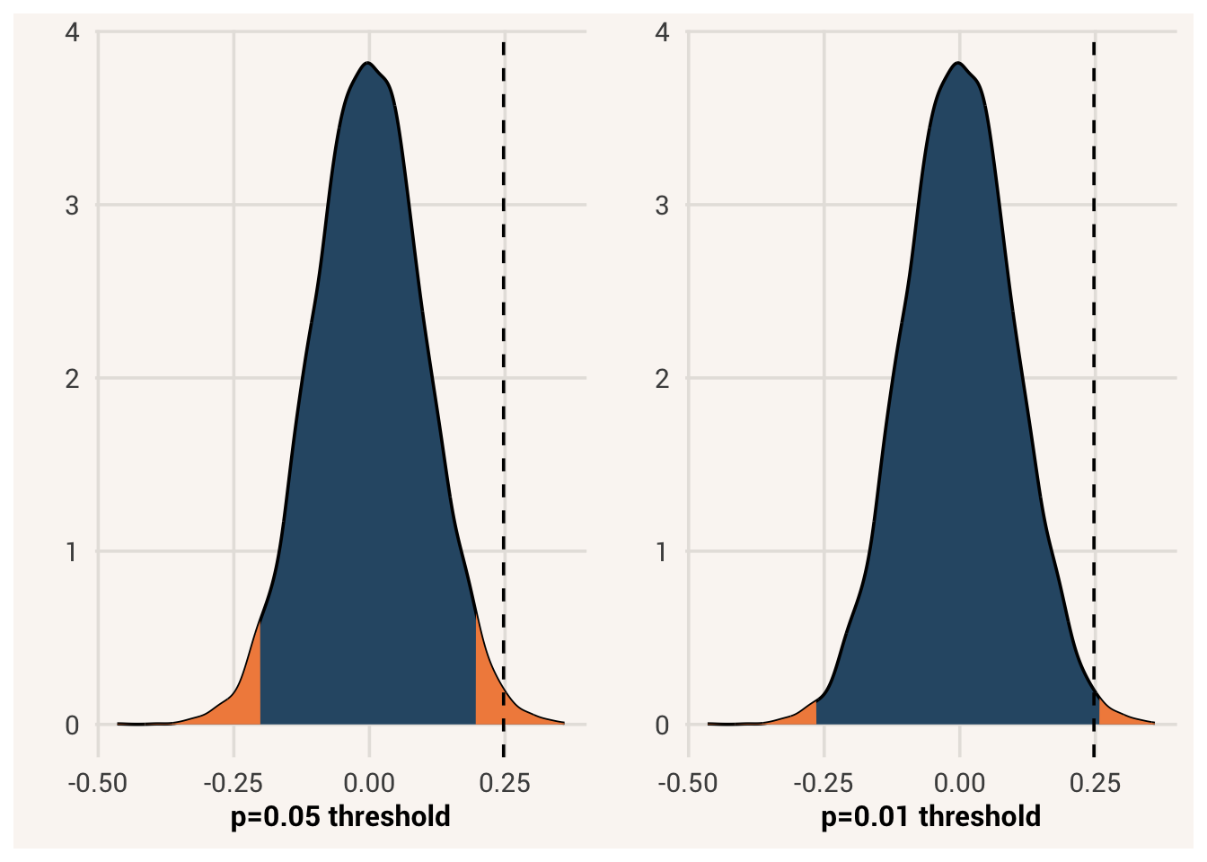
However, lowering the significance criterion can cause other problems. For instance, now imagine the real population effect is 0.2:
Now, most of the samples we get result in a positive effect estimate. But many of these estimates could also be consistent with the null hypothesis still. For instance, looking at sample 12:
In this sample, \(\hat{\beta_1}\) was estimated to be 0.1. Under the null hypothesis with a sample size of 100, that has a p-value of 0.31. 31% of the time when the null hypothesis is true, we would get an estimate as extreme or more extreme than 0.1. Thus under typical decision rules, we would fail to reject the null hypothesis even though we should have in this case, because the true population effect is not 0. Failing to reject a null hypothesis when we it is actually false is called, imaginatively, a Type II error or a false negative. When we commit a Type II error, we may throw our scientific theory away when it in fact has merit.
Type II error = in hypothesis testing, failing to reject the null hypothesis when it is false.
When we lower the \(\alpha\) criterion to reduce the chance of committing a Type I error, we increase the chance of committing a Type II error. For instance, look at sample 23:
In this sample, \(\hat{\beta_1}\) was 0.23 - that’s in fact a little bit bigger than the true \(\beta_1\) value of 0.2 in the population. Under a typical \(\alpha\) level of 0.05, we would (correctly) reject the null hypothesis. However, if we had used \(\alpha=0.01\) instead, we would fail to reject.
Thus, the significance level we choose has an influence on whether or not an estimate we calculate is judged to be significant or not. By using a larger \(\alpha\) level, we make it easier to reject the null correctly, but also easier to commit a Type I error. By lowering the \(\alpha\) level, we make it harder to erroneously reject the null, but also harder to tell when we actually should.
16.5.2 Sample size
In the simulations above, the sampling distribution of \(\hat{\beta_1}\) estimates was pretty wide. That’s because a sample size of N=100 is not all that large, and thus sample estimates are more variable. That means an estimate like -0.12 can still plausibly come from the null hypothesis, and thus is not judged as significant in a sample with N=100:
However, now imagine we actually collected samples with N=500. In the next simulation we will still set the population \(\beta_1\) to be 0, but we will collect many more observations per sample.
Our sampling distribution is much narrower now. In a narrower sampling distribution, the sample effect estimate -0.12 is much more surprising:
Now, this estimate is significant. The important difference was the sample size. When a big estimate occurs in a small sample, that isn’t too shocking because estimates from small samples can be all over the place. When a big estimate occurs in a large sample, that is much less likely to happen and is therefor more noteworthy.
16.5.3 Estimate magnitude
While we don’t have control over it, it’s important to also note and be aware of the fact that the magnitude or extremity of the estimate also affects whether or not we judge it to be significant. This has been implicit in a lot of our discussion so far, but to make it explicit - assuming the null hypothesis is true, an estimate that is farther away from the null hypothesis value is less likely to happen. If it is less likely to happen, it has a lower p-value. When that p-value falls below the significance criterion, we judge the estimate to be significant. This is why an estimate like 0.1 in the null hypothesis sampling distribution above would not be significant, but an estimate like 0.3 would be.
16.5.4 Choice of null hypothesis
Finally, our choice of the null hypothesis value also determines whether or not a particular estimate value would be significant.
So far, we have been dealing with a specific choice of null hypothesis - that the population value is 0. We’ve done this because it’s a common choice, and is the default choice in many statistical analysis packages. But sometimes there are other values we want to eliminate as possibilities for the population value. For instance, maybe we have a descriptive question like what is the marginal mean of a target variable in the population. We can model this with a null model, such as:
The one coefficient estimated for this model, \(\hat{\beta_0}\), is the mean expected leadership score for everyone before knowing anything else about them.
Usually we don’t care about an empty model like this beyond using it as a base of comparison for models with explanatory variables, but in this case it helps us answer a descriptive question about the central tendency of leadership generally. So here, our estimand is that \(\beta_0\) coefficient.
By default, this model output shows us a t-value and p-value for a hypothesis test of this estimate against a null hypothesis that the average leadership score is 0. An estimate of 3.52 is clearly significant in this context. However, it doesn’t really make sense to consider a null hypothesis \(H_0: \beta_0 = 0\) because is these data, leadership scores can never be 0 (it was measured with Likert questions on a 1-5 scale). Thus we shouldn’t be excited about rejecting \(\beta_0 = 0\) as an option for the population because it was never on the table in the first place.
Instead, we might hypothesize that the typical leadership score in our population of interest is equal to some other population’s mean value. Let’s pretend everyone in soto_work has a psychology degree, and the mean leadership score in the general population is 3.5. Thus, does our sample estimate suggest that people with psychology degrees have the same leadership score as the general population? It would be uninteresting if yes, so we’ll use the general population average as a null hypothesis: \(H_0: \beta_0 = 3.5\). We would like to reject that this is the population value our sample came from and instead believe our sample came from some other \(\beta_0\) value.
To change the value of the null hypothesis our model estimate is tested against, we need a new R package. marginaleffects makes this really easy. In this package is a function hypotheses() that takes a fitted model object as the first argument, and a second argument hypothesis= where we set what the new null hypothesis value should be.
To implement our planned hypothesis described above, we simply type:
The result shows us the \(\hat{\beta_0}\) estimate and standard error like the default summary() function does, but now it also shows us the estimate’s z-statistic (very similar to a t-statistic) and p-value relative to the new null hypothesis value of 3. Conveniently, it also shows us the 95% confidence interval of the \(\hat{\beta_0}\) estimate so we don’t need to use a different function for finding that.
While an estimate of 3.52 was significant against a null hypothesis of 0, it seems it is not significant against a different null hypothesis of 3.5. The p-value in this case is 0.42. The estimate didn’t change, but which null hypothesis we tested it against did and that influenced whether or not the estimate was judged to be significant.
16.6 Limits of null hypothesis testing
At this point you may be feeling like it’s hard to keep track of the logic of inference and hypothesis testing. That’s not uncommon; to do it well you have to hold in mind a lot of hypotheticals. There’s a hypothetical population value that would generate hypothetical sample estimates, and we need to consider where our one actual estimate falls among those possibilities. Using the null hypothesis makes that reasoning even more challenging, because we’re not actually thinking about hypotheticals generating from our actual beliefs. Rather, we’re thinking about hypotheticals that would happen if something we don’t believe in were true. Then there’s all the things that could affect our conclusion in this reasoning process, such as significance level and sample size.
Because of this convoluted thinking, it is common to make incorrect conclusions when looking at statistical inference results. In addition, there are lots of questions null hypothesis testing can’t answer for us, or situations in which the answers we get from null hypothesis testing aren’t very helpful. Thus, while a powerful option when doing inference, null hypothesis significance testing in not a panacea. Below are some of the limitations and common misconceptions of doing null hypothesis significance testing.
16.6.1 Type I and Type II error
As we saw in the previous section, we are at risk of making a Type I or Type II error when we use null hypothesis significance testing. When we use an \(\alpha\) criterion of 0.05, any estimate that is as extreme or more extreme that the far 5% values in the null hypothesis sampling distribution will be treated as unlikely and thus probably not from the null hypothesis at all. But by definition, 5% of the values in the null hypothesis sampling distribution are this level of unlikely. So when using \(\alpha = 0.05\), we may erroneously reject the null hypothesis and make a wrong conclusion.
However, while lowering the \(\alpha\) criterion reduces Type I error risk, we raise the Type II error risk. It is now harder to determine when we actually should reject the null hypothesis.
Thus Type I and Type II errors are always a tradeoff with each other - where we reduce the chance of one, we increase the chance of the other. Also, it is never possible to completely eliminate the risk of either. This is an inherent limitation of null hypothesis significance testing.
16.6.2 Hypothesis rejection, not support
A second limitation of null hypothesis significance testing is that, while it is possible to declare a sample estimate as too unlikely for us to think it comes from the null hypothesis, it is not possible to be sure an estimate definitely does come from the null hypothesis. With significance testing of one sample estimate, we can never confirm a specific null hypothesis, only reject it or fail to reject it. There are infinitely other population values slightly above or below 0 that could likely generate this estimate as well. You can’t prove that any estimate came from \(\beta_1 = 0\) specifically and not, e.g., \(\beta_1 = 0.1\). You can only say there is a very high likelihood that something did not come from a particular population value like \(\beta_1 = 0\). Null hypothesis testing is about rejecting some reality, not confirming one. If we fail to reject the null hypothesis, the true population parameter could be 0, but it could also be something else sort of close to 0. We don’t know.4
16.6.3 Significance is a binary decision
Thirdly, another limitation of significance testing is that there are not different levels of statistical significance. We can compute different p-values for different estimates and find that one has a higher probability to appear under the null hypothesis than another. But the decision of something being significantly different from 0 is a binary decision - it either is significant, or it is not. Something that is in the top 2% of the null sampling distribution is significant just as something that is in the top 0.02% of the distribution is significant, because both are beyond the \(\alpha\) cutoff. Null hypothesis testing doesn’t give us a way to test whether different p-values are significantly different from each other. Thus a sample estimate is either significant, or it’s not. We decide it either didn’t come from the null hypothesis, or there’s not enough evidence to decide. You can’t have one estimate that is more or less significant than another, and you can’t have something that is almost significant.
16.6.4 Probability of data, not population
Fourthly, the specific meaning of a p-value can be tricky to get right. It is the probability that, given the null hypothesis is true, we would find a sample estimate as extreme or more extreme than the one we did. Thinking in terms of conditional probability again, it is \(P(\hat{\beta_1} \geq b_1 | \beta_1 = 0)\). A p-value is NOT the probability that the null hypothesis is true. In Frequentist statistics, a population value cannot have a probability - it exists as a single entity that can’t be repeated multiple times like a sample. The null hypothesis thus does not have a probability. This estimate has a probability, given the null hypothesis is true.
16.6.5 P-values and sample size
Lastly, as we explored previously, the p-value we get is tied to our sample size. In small amounts of data, we would need to estimate a really large effect in order to call it significant, because the null hypothesis sampling distribution is so wide that it can produce many values beyond 0. Thus when we only have a small amount of data available to us, we can declare almost nothing as significant.
But conversely, in large amounts of data almost everything is significant - even effects so tiny that they’re not useful in the real world. Would it matter to you to hear that a variable in a model was significant, but the model only explained 0.01% of the variation in the outcome data?
P-values can thus be “gamed” with large sample sizes. They tell us something about whether our estimate could plausibly occur under the null hypothesis, but they don’t help us with determining whether a tiny-but-technically-not-zero effect is useful for real-world purposes.
In summary, there are five main hang-ups that cause a lot of consternation for people trying to use null hypothesis testing:
The risk of Type I and Type II error is everpresent
You can only reject the null hypothesis, or fail to reject the null hypothesis (not confirm the null hypothesis)
You can only decide if a sample estimate is significantly different from 0 or not; there are no levels of significance
A p-value is the probability of these data given the null hypothesis, NOT the probability of the null hypothesis given these data.
P-values are tied to sample sizes, so it is possible to miss true effects in small datasets and to get a significant p-value with an impractically-tiny effect in large datasets.
This is a long section on the difficulties of null hypothesis testing because a lot of people use it incorrectly, even professional scientists. Null hypothesis significance testing is a powerful approach, but it’s tricky to interpret correctly and it often gets used for the wrong questions that it is just not able to answer.
Thus if you default to only ever looking at p-values in your research and not the wider context of what your model looks like and what goals you have for it, you run the risk of misinterpreting your statistics. Just because a p-value is significant does not mean your model can be used in the way you want to. We’ll cover the idea of practical vs. statistical significance in a later chapter but for now, remember that p-values aren’t the whole story! We also want to judge how well our models fit a dataset, the effect size of the estimates in a model, and precision of those estimates.
16.7 Chapter summary
16.7.1 Learning goals
After reading this chapter, you should be able to:
- Specify a null hypothesis for an estimand’s value
- Define and find a p-value of an estimate
- Interpret the significance of an estimate, given a null hypothesis and significance criterion
- Explain the limits of null hypothesis testing
16.7.2 New concepts
- hypothesis testing: the process of comparing real data to hypothesized expectations as a way of deciding whether the expectations were good or not.
- t-statistic: standardization of an estimate relative to its sampling distribution, calculated as the difference between the estimate and sampling distribution mean divided by the estimated standard error.
- p-value: the probability of getting a sample estimate as extreme or more extreme than a calculated estimate, assuming the hypothesized population value is true.
- statistical significance: a large enough difference between a hypothesized estimand value and one’s estimate that makes one reject the hypothesized value.
- significance criterion \(\alpha\): the level of probability used for making a decision of statistical significance about an estimate; if the probability of getting our estimate or more extreme is less than the significance criterion, significance is decided and the hypothesis rejected.
- null hypothesis: a hypothesis that the value of a population estimand is not a particular value.
- F-distribution: a probability distribution of estimates that is bounded at 0 and has a long tail to the right.
- Type I error: in hypothesis testing, rejecting the null hypothesis when it is true.
- Type II error: in hypothesis testing, failing to reject the null hypothesis when it is false.
16.7.3 New R functionality
Standard error is clculated different ways for different estimands. For a model coefficient \(\beta_j\), it is \(\sqrt{\frac{VIF_j * \Sigma(y_i-\hat{y_i})^2}{(n-k-1)*\Sigma(x_ij-\bar{x_j})^2}}\), where VIF is the variance inflation factor of a variable.↩︎
More verbosely, this is a two-sided p-value. It’s also possible to calculate the probability of getting only an extremely high or extremely low score, but that’s less common.↩︎
“Pr(>|t|)” stands for the probability of drawing an estimate from the sampling distribution that has an absolute t-value at least as large as ours.↩︎
Note that there is a way to build support for the null hypothesis in Frequentist statistics, called equivalence testing, but it uses a different approach.↩︎